Complement (negation): Ac = { x
Reflection (transposition): Ar = { x
Intersection of A and B: A
Union of A and B: A
Difference between A and B: A-B = {x
Contents:
Morphology (the study of the form of obejcts) is an important basis for image processing. It simplifies an image by removing irrelevant details and errors with which the essential characteristics of the form of objects remain intact. The objects can easily be recognized.
Morphological operations are often used in machine vision and robotic applications. The basic operations of mathematical morphology are: dilation, erosion, opening and closing. These can be applied to both binary and gray value images. There are hardware implementations (especially for 3*3 or 5*5 operations) which work at video speed.
For an overview on morphology see: R. Haralick, S. Sternberg, X. Zhuang: Image Analysis using Mathematical Morphology. IEEE PAMI 9, 532, (1987)
Set theory is the mathematical basis for morphology. Sets in Euclidic space E2 (or rather Z2 : the set of pairs of integers) describe the object pixels in a binary image, either the black or white pixels. Z3 sets are used for describing the 3-D or time series of 2-D binary images as well as 2-D gray level images.
Elementary operations [fig 9.1 and 9.2] on A: a subset or En with n-tuple elements a=(a1,a2,...an).
Translation over d![]() En: Ad = { x
En: Ad = { x![]() En | x = a + d, for some a
En | x = a + d, for some a![]() A}
A}
Complement (negation): Ac = { x![]() En | x
En | x ![]() A }
A }
Reflection (transposition): Ar = { x![]() En | x =
-a, for some a
En | x =
-a, for some a![]() A}
A}
Intersection of A and B: A ![]() B = {x
B = {x![]() En | x
En | x ![]() A and x
A and x ![]() B}
B}
Union of A and B: A ![]() B= {x
B= {x![]() En | x
En | x ![]() A or x
A or x ![]() B}
B}
Difference between A and B: A-B = {x![]() En |
x
En |
x ![]() A and x
A and x ![]() B} = A
B} = A ![]() Bc
Bc
 |
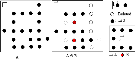
The dilation operator on sets A and B are defined by: A A is normally the image, while B is often a smaller structuring element. |
 |
 |
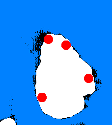
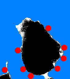
Dilation with a discrete "disk", the origin being inside of it, gives an isotrope "swelling" or "expansion" of the image; see also fig. 9.5. On the left is the original image (from Tutorial Mathematical Morphology) , on the right the result after swelling; note that here the white pixels have been chosen as the object pixels. |
 |
On the disk on the left some places have been marked red, black indicates the original pixels and white the pixels that were added in. This implementation is based on an equivalence definition of dilation: A Br is placed on each pixel x of the image and if there is at least one pixel in A in Br then x belongs to A Dilation with a 3*3 square, containing the origin, is called "fill", "expand" or "grow", see [fig 9.4]. |
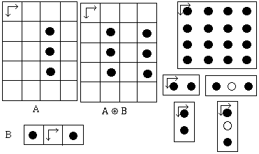 |
Dilation is communitative and associative: A This is used in software and hardware implementations to save on operations; if B and C each have N elements then this can have B On the far right you can see that dilation can be done using a 4 by 4 square with 16 pixels, with 4 consecutive dilations, and with 4 structure elements each with 2 pixels. To the left you can see
that if the origin is not in B, then it is possible that A |
Furthermore it can be shown that:
A ![]() B =
B = ![]() [b
[b![]() B] Ab and
Ad
B] Ab and
Ad ![]() B = (A
B = (A ![]() B) d and Ad
B) d and Ad ![]() B-d = A
B-d = A ![]() B
B
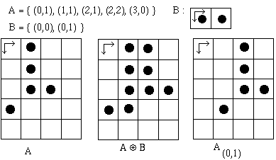
The first equation can be seen in the first figure of this section, where B contains the elements (0,0) and (0,1) and A ![]() B = A(0,0)
B = A(0,0) ![]() A(0,1) = A
A(0,1) = A ![]() A(0,1). These equations form the basis for the implementation of dilation using the digital hardware
available on many image-processing cards. Shifts in the operation pipeline can then be compensated by scrolling the output buffer.
A(0,1). These equations form the basis for the implementation of dilation using the digital hardware
available on many image-processing cards. Shifts in the operation pipeline can then be compensated by scrolling the output buffer.
The following equations can be used for a quicker implementation:
(A ![]() B)
B) ![]() C = (A
C = (A ![]() C)
C) ![]() (B
(B ![]() C) and A
C) and A ![]() (B
(B ![]() C) =
(A
C) =
(A ![]() B)
B) ![]() (A
(A ![]() C)
C)
For the combination of intersection and dilation the following is true:
(A ![]() B)
B) ![]() C
C ![]() (A
(A ![]() C)
C) ![]() (B
(B ![]() C) and A
C) and A ![]() (B
(B ![]() C)
C) ![]() (A
(A ![]() B)
B) ![]() (A
(A ![]() C)
C)
Furthermore the dilation increases:
A![]() B
B ![]() A
A ![]() C
C ![]() B
B ![]() C for an image and A
C for an image and A![]() B
B ![]() C
C ![]() A
A ![]() C
C ![]() B for a structure element
B for a structure element
There are several equivalent definitions which can be given for erosion:
A![]() B = { c
B = { c![]() En | (c + b)
En | (c + b) ![]() A for every b
A for every b ![]() B }
B }
= { c![]() En | Bc
En | Bc ![]() A }
A }
= { c![]() En | for every b
En | for every b![]() B there is an a
B there is an a![]() A
such that c = a-b}
A
such that c = a-b}
= ![]() [b
[b![]() B] A-b
B] A-b
 |
Erosion is not commutative nor is it equal to the difference of the sets. (0,0) thus resulting in "shrinking" of the original image, see [fig. 9.6] |
 |
 |
Erosion of the same image used in the previous dilation section. |
Here follow some equations for the acceleration of hardware and software implementations:
AdB = (A
AC) = (A
(A
(ABr (erosion-dilation duality) and (A
A
Some implications:
AB
A
BC
Union and erosion: (A ![]() B)
B) ![]() C
C ![]() (A
(A![]() C)
C) ![]() (B
(B ![]() C)
C)
These operations are a combination of dilation and erosion:
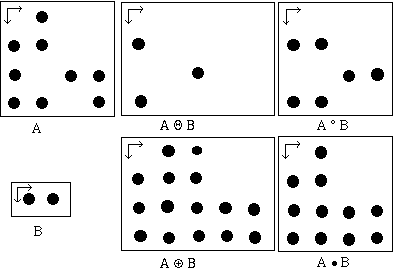
opening: AK = (A
K = (A
 |
Geometric characteristics, see [fig. 9.8 and 9.9]: A{ x representing the union of translations of B which are contained in A A representing the complement of the union of all translations |
 |
 |
To the left is the open operation on the same original from the previous section. The structure element moves along the inside of the object and the black pixels disappear. To the right is the close operation, the structure element moves along the outside of the object and the white pixels are added. |
 |
The original image (from Tutorial Mathematical Morphology), here the real pixel size is that of the small black or white blocks. |
 |
Erosion of the original image with a 3 by 3 structure element. |
 |
Followed by a dilation of the previous eroded image, thus the open operation on the original image. Two thin connections in the object have been broken. A small protrusion and a small island have been eliminated. |
 |
Dilation of the original image with a 3 by 3 structure element. |
 |
Followed by the erosion of the dilated image, thus the close operation on the original image. A hole in the object has been filled, as well as two small dents in the contour. A small hole between the two pairs of the object has been filled. |
Thus opening with a disk structure element (see fig. 9.10):
- breaks thin connections within an object
- eliminates small islands and sharp protrusions
and closing with a disk structure element:
- fills thin connections within an object
- eliminates small holes and fills dents in contours
- fills small gaps in parts of an object
From the geometric definitions of opening the following can be deduced:
B
(A
From the geometric definitions of closing the following can be deduced:
A
A
A
(A
= (A
A
From (1) and (2) it follows that: A![]() K = (A
K = (A![]() K)
K) ![]() K = (A
K = (A![]() K)
K) ![]() K (already shown
above) (3)
K (already shown
above) (3)
In the same manner the following can be deduced: A![]() K = (A
K = (A![]() K)
K) ![]() K = (A
K = (A![]() K)
K) ![]() K
K
From this follows:
A
= ((A
= (A
A
thus opening and closing are idem potent operations.
Duality of opening and closing: (A![]() K)c = Ac
K)c = Ac ![]() Kr
Kr
Furthermore, opening and closing are invariant under the translation of the structure element:
A![]() Kx = A
Kx = A![]() K and A
K and A![]() Kx = A
Kx = A![]() K
K
 |
 |
 |
 |
 |
Top left is the original image with a lot of noise, see fig. 9.11. Top right is the opening thereof with a 3 by 3 structure element, and the result of closing on that image is shown below it. The center image in the left column is the closing of the original image and below it the opening of that. |
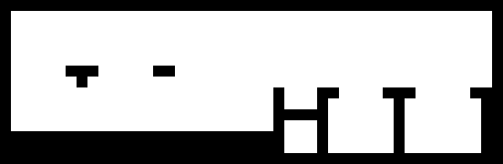
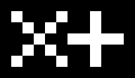
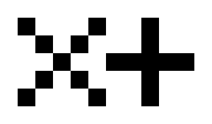
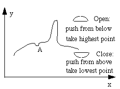
The goal of the "hit-miss" operation is to find the pixels x, for which B1x is in A and where no pixel in B2x is in A, thus
B2x is in Ac. With B1 and B2 being structure elements not having pixels in common ( B2![]() B1c ) or else the set of x will be empty. The definition of the "hit-miss" operation is:
B1c ) or else the set of x will be empty. The definition of the "hit-miss" operation is:
AB = { x
En | B1x
We thus get the pixels x for which B1x is in A ("hit") and B2x is not in A ("miss"). It can be shown that:
A
 Original image (white pixels) |
B1 |
 Erosion with B1 |
Searching for white pixels, |
 Complement |
B2 |
 Erosion with B2 |
 Intersection yields the resulting image |
Edge extraction, see [fig. 9.13]: GB(A) = A - (A ![]() B)
B)
Filling regions that are defined by a 8-connected boundary can be done by an iterative process, see [fig. 9.15]:
X0 = p (a random pixel in the region)
Xk = (Xk-1
stop the iteration when Xk = Xk-1
Xk
Finding a connected component in an image, see [fig 9.17]:
X0 = p (a random pixel of the component)
Xk = (Xk-1
 |
The thinning of a set A by a composed structure element B: usually A is thinned symmetrically by a row of structure elements {B}, that are rotated versions of each other: this is repeated until no more changes occur, see [fig. 9.21]. The center picture shows the results using {B} from fig. 9.21, the bottom one with a slightly different {B}. |
 |
|
 |
Growing (or thickening) of a set is defined in the same manner, see [fig. 9.22]:
AB = A
A
The skeleton of a region A, pixels from which the area can be built up of with the aid of structure element B, can also be defined as ( see [fig. 9.24] ):
S(A) = k=0
Sk(A)= (A
K = max{ k | A
}
A = k=0
Also protrusions of a figure, of for example less than 3 pixels, can be removed (pruning), see [fig. 9.25].
L. Vincent (Signal Processing 22,1991,3-23) gives an efficient algorithm for the implementation of morphological operations with random structure elements, assuming a chain code encoding of the binary objects.
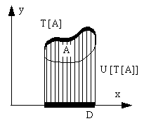 |
For morphological operations on gray level images we use sets in EN. The first (N-1) coordinates conventionally form the spatial domain and the last coordinate is for the surface. For gray level images N=3, the first two coordinates of an element in a set are the (x,y) in the image and the third is the gray level. Concepts such as top or top-surface of a set and the shadow (umbra) of a surface are used in the definitions of the operations. |
Let A be ![]() EN and define the domain of A as: D = { x
EN and define the domain of A as: D = { x ![]() EN-1 | there is a y
EN-1 | there is a y![]() E, (x,y)
E, (x,y)![]() A}
A}
The top or top-surface of A is a function T[A] : D -> E: T[A] (x) = Max { y | (x,y) ![]() A }
A }
Set B ( B ![]() EN-1
EN-1 ![]() E) is a shadow if and only if: (x,y)
E) is a shadow if and only if: (x,y)![]() B
B ![]() (x,z)
(x,z)![]() B for every
z
B for every
z ![]() y
y
Let f : D -> E be a function, then U[f] ( U[f] ![]() D
D ![]() E ) the shadow set of f: U[f] = { (x,y)
E ) the shadow set of f: U[f] = { (x,y)![]() D
D ![]() E | y
E | y ![]() f(x) }
f(x) }
Let F,K ![]() EN-1 domains and f: F -> E and k : K -> E the functions belonging
to it.
EN-1 domains and f: F -> E and k : K -> E the functions belonging
to it.
Then define dilation as ( see [fig. 9.27] ):
f
erosion is defined as ( see [fig. 9.28] ):
f
See [fig. 9.29] for the result of dilation and erosion on a gray level image. The properties of gray level dilation and erosion are equivalent to those of binary operations, for example:
(f
 |
Opening and closing are defined as follows: f To the left is the geometric interpretation of it, see also [fig. 9.30]. See fig. 9.31 for the results on the image of fig. 9.29. The duality of open and close is: -(f |
 |
 |
 |
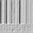
To the far left is the original image, in the center the opening of it with a disk with radius 3 as the structure element. All the thin white bands have disappeared, only the broad one remains. To the right the closing, all the valleys where the structure element does not fit have been filled, only the three broad black bands remain. The bottom row is the top view of the three images above. The images come from mmtutor. |
 |
 |
 |
Last updated on April 4th 2003 Theo Schouten.