The integral must be taken from -
Contents:
If f(x) is a 1 dimensional continuous function which can be integrated and having a real variable, then the Fourier transformed function f is defined as follows:
The integral must be taken from - to +
, the range of x. Because this is obvious I often tend to omit it due to the restrictions of HTML. The inverse Fourier transformation (if F(u) can be integrated) is:
An example: f(x) = rect(x) with rect(x) = 1 if -0.5 < x < 0.5, else 0
Then :
|
F(u) shows how much of frequency u exists in the signal f(x); f(x) is sometimes called f(t) with t being time (see fig. 4.1) This is an example from the wavelet tutorial of R. Polikar: |
|
F(u) is shown here. The 4 frequencies are clearly visible. The peaks are somewhat broader because of the interference of waves due to edging effects (it wasn't measured for an infinite amount of time). |
In general F(u) is a complex function:
F(u) = R(u) + j I(u) = | F(u) | ej(u)
| F(u) | =( R2(u) + I2(u) ) : the Fourier spectrum of f(x)
(u) = tan -1 ( I(u) / R(u) ) : the phase angle of f(x)
Here is another example:
If f(x) changes rapidly with small steps of x, then |F(u)| will be large for large values of |u|. If f(x) barely changes, in the example only in 2 places, then |F(u)| will be large for small
values of |u|.
For 2 dimensional functions there is an analog definition:
F(u,v) =f(x,y)
(ux+vy) dx dy
f(x,y) =F(u,v)
(ux+vy)du dv
 |
 |
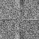 |
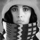
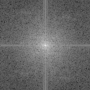
The original picture, a Fourier spectrum in logarithmic scale ( log|F(u)| ) is often used because of the large range of |F(u)| ) and the phase image. The "lines" in the spectrum and phase diagram show that there are numerous strong horizontal and vertical intensity transitions in the picture. |
| Here (images from Khoros Lab) the spectra of an image and the rotation thereof are shown. |
Shown here is in polar coordinates, the rotation of a function over a certain angle corresponds to the rotation of the Fourier transformed function over that same angle. |
Here is a graphic reproduction of the convolution operation.
A practical example of a convolution is the projection through a lens system.
A mathematical point of light is not projected as one point but rather smudged out.
The radiation of the ideal point (,
) (the Greek letters xi and eta) is spread out over the neighboring pixels (x,y) by the function h(x,
,
y,
), the spread-out-point or impulse-response function. The last term comes from the electronics world and shows
the response of a system to voltage or a current impulse. The ideal image w(
,
) is spread out evenly until the measured image becomes p(x,y) =
w(
,
) h(x,
, y,
) d
d
. During the first approximation (we then speak of a linear system) the spreading out is independent of the position of
the image surface, and thus independent of where the light enters the lens: h becomes h(x-
, y-
). The measured image then becomes p(x,y) =
w(
,
) h(x-
, y-
) d
d
, and thus a convolution of the ideal image with h. In the Fourier space: P(u,v) = W(u,v)H(u,v), using P and H it is
easier to calculate W en thus w.
|
|
A digital image is not a continuous function but rather just a row (1-D image) or a matrix of numbers. We also want a Discreet Fourier transformation (DFT) on that. Imagine there is a continuous function g(x) with G(u) its Fourier transformed function. Take a row of values from g as follows:
{ f[0], f[1]...f[N-1] } = { g(x0), g(x0+x)...g(x0+(N-1)
x) }
and define the discreet Fourier transformation as:
F[u] = 1/N x=0N-1 f[x]
xu / N for u=0,1...N-1
f[x] = x=0N-1 F[u]
xu / N for x=0,1...N-1
The scaling factor 1/N can be chosen differently, for example 1/N with F(u) as well as f[x].
One can then show that the following holds:
{ F[0], F[1]...F[N-1] } = { G(0), G(u)...G( (N-1)
u) } with
u= 1 / (N
x)
so the DFT of a row of values taken from the function g results in a row of values in G. It holds that for every row of numbers appropriate continuous functions g and G that can be differentiated can be constructed. Many properties of FT and DFT will therefore be analogous.
In 2-D the DFT becomes:
F[u,v] = 1/MN x=0M-1 y=0
N-1 f[x,y]
(xu / M + yv / N)
f[x,y] = u=0M-1 v=0
N-1 F[u,v]
(xu / M + yv / N)
With square images (M = N) the scale factors 1/MN and 1 are usually chosen as 1/N and 1/N.
A 2-D DFT can be calculated as 2N 1-D DFTs:
F[x,v] = 1/N y=0N-1 f[x,y]
yv / N for x=0,1...N-1
F[u,v] = 1/N x=0N-1 F[x,v]
xu / N for v=0,1...N-1
| The u and v are always positive in the 2-D DFT, we therefore look at the first quadrant of G(u,v), the FT of the continuous function g(x,y) that corresponds to the matrix f[x,y]. However, we want to inspect the region around the origin of G(u,v) [see also fig 4.34], because this gives a deeper understanding of it. We must then shift u and v over -N/2. From the translation properties of the DFT given above, it follows that we can take the DFT of the matrix f[x,y](-1)x+y to get G(u-N/2, y-N/2). Software packets often name this DFT, pay close attention to this and the scaling factors when combining multiple packets. |
The convolution and correlation theorems also hold for the DFT. The discrete convolution is defined as:
f[x] g[x] = m=0
M-1 f[m] g[x-m] with M=A+B+1 where A,B are the lengths of f and g, and the rows f and g are additionally filled with 0s until their lengths are M. In the equation the
indices taken modulo M.
|
In matrix notation the DFT is as follows: F = M f with the elements of M being equivalent to m n,i = 1/N |
A FFT can be implemented parallel on a multiprocessor system or with the aid of special hardware. There are special chips for the hardware implementation of a FFT, these contain tables for the exponential functions and hardware for the ordering of the elements of f[]. Computer cards can be purchased with special hardware and software, with which you can execute the 1-D and 2-D FFT quickly.
|
Using an x-ray source one can calculate the x-ray permeability of an object for the amount of generated radiation. A simple model for these measurements is the projection of the 2-D attenuation
function f(x,y) on the x-axis under an angle of g |
A large amount of 1-D projections g(x') are measured. If we look at
= 0, thus the projection on the x-axis, and we take the FT:
FT( g0(x')) = (
f(x,y) dy)
xu dx =
f(x,y)
xu dx dy = F(u,0)
This can be generalized to: FT( g(x')) = F(u cos
, u sin
).
|
With discrete data we can find the points (u cos In practice many problems arise in the following situations: tendency of the source's radiation to diverge, the radiation not being uniform, or the slice having locations with a high absorbency which leaves a shadow: the absorption in the rest of the strip isn't of interest anymore. There are also problems with aliasing (see chapter 2.4.4) during interpolation in the FT space. |
|
With the reciprocal projection method the recording area is split up into pixels (with a dimension smaller or equal to that of the source or recording element size). Every measurement is simply distributed proportionally over every contributing pixel. In the example on the left we only distribute over entire pixels; in practice we must also distribute over partially contributing pixels. The result of the distribution of the four projections (the appointed values averaged) is shown in the bottom square; it does not approximate the original values very well. |
Let's look at the reciprocal projection reconstruction of the point source. With n reciprocal projections, 2n points lie on the circumference of a circle with radius r, this is a density of
2n/2r. The point is smeared out to a smudge by a now known point-spread function. Thus the image g is a
convolution of the real image f with the point-spread function: g(x,y) = f(x,y)
h(x2 +
y2) and in the Fourier space: G(u,v) = F(u, v) H (u, v). By multiplying G(u, v) with H-1 we can calculate F(u,v) and f(x,y) by the reciprocal transformation. The function h(r)
must be chosen carefully (the FT must exist), by for example stopping at a low r.
Because the operations applied are all linear, the deconvolution can first be applied to the projection data followed by the reciprocal projection. This is faster and efficient because the deconvolution can occur while data acquisition of the following line takes place. In practice, this filtered reciprocal projection works the fastest and knows no convergence problems, but often introduces errors around sharp objects due to interference of the virtual pattern with the filter pattern.
|
With the algebraic iterative reciprocal projection, every projection value is distributed over the (partially) contributing pixels according to the values that the pixels obtained in the previous step. As can be seen with our simple example, we can already get a quick and decent approximation of the real intensity distribution. Convergence problems often arise which can in turn be dealt with heuristically. However, this can lead to many problems if the signal to distortion ratio is very poor. |
In practice, see Imaginis Corp, the geometry of the measurements and thus the model that must be followed and calculated, is much more complicated. |
See for example Aracor for non-medical applications of CT scans. Here is an example of non-destructive measurements of a casted aluminium object. The measured wall thickness in the CT scan coincides well with the physical measurements. |
The DFT is an example of an entire class of image transformations in 1-D and 2-D:
T(u) = x=0N-1 f(x) g(x,u) with g the forward transformation kernel
f(x) = u=0N-1 T(u) h(x,u) with h the inverse transformation kernel
T(u,v) = x=0N-1 y=0
N-1 f(x,y) g(x,y,u,v)
f(x,y) = u=0N-1 v=0
N-1 T(u,v) h(x,y,u,v)
If g(x,y,u,v) = g1(x,u) g2(y,v), then the 2-D transformation is separable and can be calculated as 2N 1-D transformations. If g(x,y,u,v) = g1(x,u) g1(y,v), then the transformation is called symmetric and is naturally also separable. Using the DFT, both the forward and the inverse transformation kernel are separable and symmetric.
As examples of these transformations the book gives the Walsh-Hadamard and the discrete cosinus transformations. The Discrete Cosine transformation (DCT) has often been used for image compression (JPEG and MPEG) over the last few years:
C(u) = (u) x=0
N-1 f(x) cos( (2x+1)u
/ 2N)
f(x) = x=0N-1
(u) C(u) cos( (2x+1)u
/ 2N)
with t (u) =
(1/N) for u=0,
(2/N) for u>0
The Hotelling transformation, also known as eigenvector, principal component or discrete Karhunen-Loeve transformation, is based on the statistical properties of vector representation. It calculates the eigenvectors and eigenvalues of the covariance matrix of the pixels and transforms the image, see chapter 11.4. The most information is located in the axis with the highest eigenvalue, these can be used for example for object recognition or image compression.
|
The FT acts as if the frequencies occur in the entire image, as in example 3.1. However, a wave can also occur locally, as shown here. The same four frequencies as in 3.1 occur but each only occurs in a quarter of the image. |
|
In this FT the same frequency peaks occur as in the FT in 3.1. However, these are broader and there is more background; this is caused by the transition between the waves, for which frequencies are to describe. With the Short Term Fourier Transform (STFT) the FT is determined for each x in a region around x: STFTw(x,u) = |
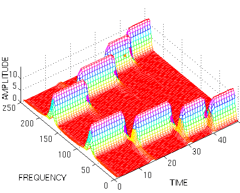 |
The STFT can be shown in a 3-D plot, a time-frequency distribution for example (this is not the STFT of the figure shown above, the symmetry occurs with each FT and is often omitted). |
|
Wavelets, or small waves, are an example of MRA. Here the scaling and the position of the frequency analysis are placed in the transformation kernels. With Continuous Wavelet Transformation (CWT)
we assume having a basis wavelet g(x) with the property Cg = |
|
(a) Morlet wavelet with random width and amplitude, with time represented along the x-axis. |
From this a set of wavelet basis functions gs,t(x) are derived:
gs,t(x) = g( (x-t) / s) /s, with s > 0 the scale and -
< t < +
the translation.
The CWT of f(x) L2(R) (so
|f(x)|2 dx <
) is then:
Wf(s,t) = <f, gs,t> =f(x)gs,t(x) dx ( <,> gives the inproduct)
The Ws can be used to determine the f again:
f(x) = (1 / Cg )Wf(s,t) gs,t(x) dt ds/s2 (the
over s is from 0 to
)
|
A g(x) with a separate frequency in each quarter and the CWT thereof. |
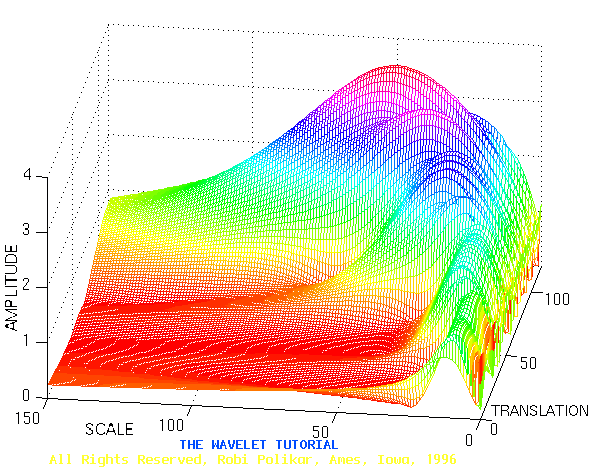
|
In the figure above the peaks are smaller at a smaller scale than at a larger scale. The scale resolution is thus lower at a smaller scale value. Because a scale value is proportional to the inverse of the frequency, higher frequencies have a worse frequency resolution than lower frequencies. This is represented graphically in the additional figure. Every rectangle has a region in the frequency-time space and that in its whole contributes to one value of Wf. With small (respectively large) frequencies there is a small (respectively large) dispersal in the frequency and a large (respectively small) dispersal in x or t. Using the STFT every rectangle would have been equal in size. |
The CWT can also be described as a convolution. Define a basis wavelet function with a scale s as: gs(x) = g(x/s) / s (taking t=0 ) and g-s(x) = g*s(-x) where * indicates the complex conjugated function. Then the following holds:
Wf(s,t) =f(x) g-s(t-x) dx = f
g-s
Thus for a static s, Wf(s,t) is the convolution of f(x) with the reflected conjugated wavelet at a scale s.
With the 2-D CWT there are 2 translation values:
gs,tx,ty(x,y) = g( (x-tx) / s, (y-ty) / s) / |s|
Wf(s,tx,ty) = <f, gs,tx,ty> =f(x,y)gs,tx,ty(x,y) dx dy
With dyadic wavelets we confine ourselves to the binary (factors of 2) scaling and dyadic translations:
gj,k(x) = 2j/2 g(2jx-k) with j,k integers in the range -to +
that form an orthogonal basis of L2(R):
<gj,k , gl,m> =j,l
k,m with
the Kronecker delta function
and where for each value f(x) L2(R) the following holds:
f(x) =j
k cj,k gj,k(x)
cj,k = < f, gj,k> = 2j/2f(x) g(2jx-k) dx
If f(x) has a limited range where the function is not equal to 0 and g(x) is localized well (that is: rapidly goes to 0 when x deviates from 0), then many cj,ks will have become neglectably small for large values of |k|. The coefficients with large |j| will be small because the wavelet is either extremely slim or broad. The series expansion of f will then have a limited amount of relative terms.
With compact dyadic wavelets we restrict ourselves to f(x) and basis wavelet functions that have the value 0 outside of the interval [0,1]. The scaling and translation can then be pinpointed by one integer n >= 0:
g0(x) = 1
gn(x) = 2j/2 g(2jx-k) for n>0, with n= 2j + k and j the largest integer such that 2jn
f(x) =n cn gn(x) with n= 0...+
The simplest compact dyadic wavelet is the Haar wavelet given by:
g(x) = 1 if 0x<0.5 and -1 if 0.5
x<1 and of course 0 outside of those intervals.
The discrete wavelet transformation (DWT) can be derived from this by sampling N points f[i] from f(x) and every gn(x):
cn =i f[i] gn[i] and f[i] =
n cn gn[i] for i,n = 0...N-1
There are 3 older techniques that have resulted in the development of DWT: filter bank theory, multi-resolution of time-scale analysis, and especially applying pyramid representations and sub band coding. These also give insight on how to construct appropriate wavelets for certain applications. There is also a fast DWT (FWT) designed with a complexity of O(n), thereby faster than the FFT.
Wavelets are used for compressing images, for improving images and for image fusion: the combining of two or more images to one resulting image. The latter is used for medical images that have been acquired using different techniques, for example the CT, MRI or PET.
Updated on January 23th 2003 by Theo Schouten.