g(x,y) = FT-1[H(u,v) F(u,v] = h(x,y)
Contents:
Techniques for editing an image such that it is more suitable for a specific application than the original image is generalized as image enhancement. The quality of the improvement can thereby actually only be graded in relation to the particular application domain: in how far does the image improvement result in an improvement in that particular application. Image enhancement methods are used like all other methods and algorithms in image processing, as a chain subsequent edits aimed at achieving a suitable result. Improving one link in the chain is only useful if the end result is really improved, and that does not solely depend on that particular link; it also depends on all the other links and the quality of the first image.
This makes quality assessment of the algorithms in image processing so difficult. Too often in scientific publications you see that the new methods or algorithms are only applied to one or a few images. The resulting image is then shown adjacent to the result of the other method; the author then claims his method to be better. This is a general portrayal of computer science, there is too little experimental evaluation of ideas. For more information see the article: "Experimental Evaluation in Computer Science: A Quantitative Study " by Paul Lukowicz, Ernst A. Heinz, Lutz Prechelt, Walter F. Tichy, Journal of Systems and Software 28(1):9-18, January 1995 and "A Quantitative Study of Experimental Evaluations of Neural Network Learning Algorithms: Current Research Practice" Neural Networks 9(3):457-462, April 1996:
| 0 | 1 | 2 | 3 | 4 | 5 | >=6 | |
| different problems | 3 | 39 | 25 | 18 | 6 | 4 | 5 |
| realistic or real problems |
29 |
41 |
16 |
7 |
3 |
2 |
2 |
| compared algorithms |
33 |
35 |
13 |
5 |
5 |
6 |
3 |
In the first row we show the percentage of articles that tested the presented algorithm on 0 to 6 or more other problems (artificial, realistic or real), in the second row those tested on realistic or real problems and finally, the percentage that compares the algorithm with 0 to 6 or more other algorithms.
In image enhancement people often use "spatial redundancy": pixels close to each other often contain almost the same information. Of course this is not true at the edges of objects or with surfaces having a very strong texture, these cases must be signaled and deserve extra attention.
Characteristically of image processing is that not much use is made of higher level, internal model information about the portrayed scene. Whether it is a car, a face or a stream of blood in the heart that is portrayed, it isn't of much interest to the image enhancer, but it is for the amount of noise or distortion in the image. In the spatial domain the methods can often be implemented as parallel edits on spatial local information (e.g. a pixel and its 8 neighbors). It is then often possible to quickly implement it on special hardware.
In the spatial domain the image enhancements can be modeled as: g(x,y) = T[f(x,y)]
the transformation T is defined over the neighborhood of (x,y), often a square ( 3*3 or 5*5) area. This has many synonyms: mask, template, window or filter editing. T can be either a linear or a non-linear edit. For a 1*1 neighborhood it becomes the gray level or color level transformation s = T(r), also named point processing.
Image enhancement can also be done in the frequency domain:
g(x,y) = FT-1[H(u,v) F(u,v] = h(x,y) ![]() f(x,y)
f(x,y)
where FT-1 is the inverse Fourier transformation, H(u,v) is called the transfer function and h(x,y) is called the spatial convolution mask, impulse response or point spread function. Image enhancement is always a linear operation in the frequency domain.
Sometimes it is better understood or described what an operation actually does in the other of the two domains. For implementation one uses the domain in which the operation can be executed the fastest, keeping in mind what other operations must also be executed.
These manipulations transform gray values or color values into other gray- or color values. Gray, and also color values are usually indicated by a 2-D plot with horizontally the old gray value and vertically the new value.
 |
In the left plot the points (r1,s1) and (r2,s2) check the changes in gray level. Gray levels between r1 and r2 are reproduced in a larger range than between s1 and s3; this is called contrast
stretching [see fig. 3.10]. If r1=r2, s1=0 and s2 = L-1 the image is translated into a binary image, an image having only 2 gray levels. This translation is called thresholding, r1=r2 is
called the threshold. |
 |
 |
Gamma transformations are of the form s=cr |
Many machines used for the acquisition, printing or viewing of images have a relationship between input and output intensity (and color) according to the "power-law". Nowadays this is often, especially with expensive machines, corrected according to a "profile" such that realistic images can be made.
 |
|
With histogram equalization we search for a T(r) that makes the histogram as smooth as possible, because that often gives a better image. The T(r) that accomplishes that is:
sk = round( L j=0k (nk / n) )
with nk the number of pixels with gray level k, n the total number of pixels and L the number of gray levels.
A histogram where j=0![]() k nk instead of nk is plotted out, is
called an accumulated histogram. For the interested, the derivation of this formula is given in the book in section 3.3.1 (page 91).
k nk instead of nk is plotted out, is
called an accumulated histogram. For the interested, the derivation of this formula is given in the book in section 3.3.1 (page 91).
 |
|
 Original |
 Contrast stretched |
 Hist. equalizations |
 Local histogram |
 Local contrast |
Above is an example from Image Processing Fundamentals with from left to right: the original image, the contrast stretched image with the lowest gray level mapped onto 0 and the highest to 255, the histogram equalized image, the local histogram equalized image and the adaptive contrast image.
Histogram equalization can also be applied locally. For each pixel the histogram is taken of a certain region around it, for example 7*7 or 9*9 pixels. The T(r), which equalizes the histogram, is determined and the new pixel value becomes the T(r) of the old value. See also fig. 3.23 for an appropriate image to apply this to.
Instead of histograms one can also look at other characteristics of intensity distributions in the neighborhood of a pixel, for example:
g(x,y) = kM ( f(x,y) -(x,y)) /
(x,y) +
with
M is the average gray level value in the entire image; k a scaling parameter with 0 < k < 1
Here the local contrast is enlarged, see the illustration above. See fig. 3.24 to 3.26 for another use of ![]() en
en
![]() .
.
In certain situation images can be averaged to reduce noise. Assume that:
gi(x,y) = f(x,y) +i(x,y) with uncorrelated noise and an average value of 0
g(x,y) = 1/M i=1
then the following holds: E{g(x,y)} = f(x,y) and ![]() 2(g(x,y))= 1/M
2(g(x,y))= 1/M ![]() 2(
2(![]() (x,y))
(x,y))
The average image thus approximates the original image f(x,y) and the noise is a factor ![]() M smaller
than in the first image. See [fig. 3.20] for an example.
M smaller
than in the first image. See [fig. 3.20] for an example.
 |
This is used for the blurring of an image: the removal of small details and the filling in of small gaps in lines, contours and planes, and also reduces the noise in an image. The intersections of the accompanying filters are shown here on the side. |
In the frequency domain smoothing becomes: G(u,v) = H(u,v)F(u,v). Removal of high frequencies occurs by multiplying by the H(u,v) function, which goes to 0 for large values of (u,v). This is
called a Low Pass Filter (LPF) because the low frequencies are let through. In the spatial domain smoothing is the removal of drastic changes by averaging the gray levels in a certain region with a
positive weight.
 |
 |
The ideal LPF (see fig. 4.10) is given by:
H(u,v) = 1 if(u2+v2)
D0 and 0 outside, D0 is the cutoff frequency.
(the figure to the top left shows the 1-D case). The term ideal comes from the analog signaling technique, it was difficult to realize such a sharp cutoff frequency. For image processing the ideal LPF is not ideal because of the occurrence of "rings" in the spatial domain (see also fig. 4.12). This happens because the FT-1 of H(u,v) is a sinc function ( sinc(x) = sin(x) / x), see [fig. 4.13].
The Butterworth LPF: Hn(u,v) = 1 / (1+( ![]() (u2+v2) /
D0 )2n ) see [fig. 4.14] and the figure to the top right
(u2+v2) /
D0 )2n ) see [fig. 4.14] and the figure to the top right
the Exponential LPF: Hn(u,v) = exp( -![]() (u2+v2) / D0 )n
)
(u2+v2) / D0 )n
)
and the Gaussian LPF: H(u,v) = exp( - (u2+v2) / 2 D02) see fig. 4.17
allows higher frequencies to pass in limited amounts and less rings can be seen in the spatial domain (see fig. 4.15 and 4.18).
 |
|
In the spatial domain the simplest example of smoothing is the average or uniform filter:
g(x,y)= (
The filter can be shown as a convolution mask, for example for an average 5*5 filter
| 1 1 1 1 1 | 9 9 9 0 0 0 . . . . . . . . . . . .
| 1 1 1 1 1 | 9 9 9 0 0 0 . 8 5 3 0 . . 9 9 0 0 .
(1/25)| 1 1 1 1 1 | 9 0 9 0 0 0 . 8 5 4 1 . . 9 9 0 0 .
| 1 1 1 1 1 | 9 9 9 0 9 0 . 8 5 4 1 . . 9 9 0 0 .
| 1 1 1 1 1 | 9 9 9 0 0 0 . 9 6 4 1 . . 9 9 0 0 .
9 9 9 0 0 0 . . . . . . .
. . . . .
(convolution mask) image average filter median filter
With the exception of one, to the right the effect is shown of a 3*3 averaged filter on the image. The pixel values strongly deviating due to noise, 9 surrounded by 0's (and respectively 0's surrounded by 9's) are filtered away nicely to 1's (respectively 8's) in a 3*3 region. But a real edge: 9 9 0 0 becomes blurred to: 9 6 3 0; the spatial redundancy obviously does not hold in that case. See also [fig. 3.35] for an example. The median filter will be discussed later.
Sometimes we use weighed-filters, where not all the pixels have an equal weight:
|0 1 1 1 0| |1 2 3 2 1| |1 4 6 4
1|
|1 1 1 1 1| |2 4 6 4 2| |4 16 24 16 4|
(1/21) |1 1 1 1 1| (1/81) |3 6 9 6 3| (1/256) |6 24 36 24 6|
|1 1 1 1 1| |2 4 6 4 2| |4 16 24 16 4|
|0 1 1 1 0| |1 2 3 2 1| |1 4 6 4
1|
The left filter is sometimes called a round averaged filter. The right filters are (just as the square averaged filter) examples of separable filters, they can be executed as a convolution with
(1/9) | 1 2 3 2 1 | respectively. (1/16) | 1 4 6 4 1 | in the x direction, followed by a convolution in the y direction. This can be used to speed up implementation. The
filter completely on the right is a poor approximation of the Gaussian function g(x,y) = c exp( (x2+y2) / 2 ![]() 2), better approximations are not separable.
2), better approximations are not separable.
To restrict the blurring of a real edge with the average filter, one could replace a pixel value by the average value only if the pixel value deviates very much from the average:
g(x,y)= (
The threshold value T can be constant or adaptively chosen per pixel, as for example 2![]() with
with ![]() the dispersal of gray levels in the region s.
the dispersal of gray levels in the region s.
We then obtain a so called non-linear filter that cannot be executed as a convolution ( ![]() swij pij). These leave structures such as edges and lines more intact.
swij pij). These leave structures such as edges and lines more intact.
With a "rank" or "order-statistics" filter, the pixel values in the neighborhood are sorted according to increasing value, the value at a fixed position in the row is chosen to replace the central pixel. Choosing a value in the middle results in a so-called median filter (see above). The edges are less vague than with the mean filter and strongly deviating noise pixels are completely filtered out.
An example from Image Processing Fundamentals
 original |
 5*5 mean |
 Gaussian |
 5*5 median |
original |
 impulse noise: 20% of the pixels set to white |
 5*5 mean |
 5*5 median |
A median filter is especially useful if impulse or salt-and-pepper noise is present, see also fig. 3.37.
The additive J.S. Lee filter is a statistical, non-linear filter:
g(i,j) =
with ![]() and
and ![]() the average and the standard deviation of the gray levels in the examined neighborhood of (i,j), K is a constant. When K is large the following holds: g(i,j) =
the average and the standard deviation of the gray levels in the examined neighborhood of (i,j), K is a constant. When K is large the following holds: g(i,j) = ![]() , and when K is small the following holds: g(i,j) = f(i,j).
, and when K is small the following holds: g(i,j) = f(i,j).
 |
Ron Schoenmakers (a promovendus of mine) and Jacques Stakenborg have designed a morphological filter, based on the form of the intensity dispersal in the region of the central pixel. The gray levels in a 3*3 window are sorted. A line is drawn through the lowest and the highest gray levels (the local minimum and maximum). The points with the maximum local vertical distance to the line are determined. A descending line is called slope, an ascending line a segment. The endpoints of every slope or segment belong to it. The central pixel lies on one or more slopes or segments (i..i+n). The are several possibilities for smoothing: (a) average the gray levels i...i+n; (b) average the gray levels i...i+n if this is a segment, otherwise take the closest gray level of a segment pixel; (c) repeat the morphological analysis for all the slopes and segments until the minimum segment length has been found, then average over a segment or slope and the closest segment. These filters retain extremely fine structures, but were also designed for filtering mixed edge pixels out which appear in satellite photos. |
 |
This is used to bring fine details to the front of the image and to sharpen the edges of objects. In the frequency domain sharpening is achieved by: G(u,v) = H(u,v) F(u,v). Removal of low frequencies through multiplication with a H(u,v) function which goes to 0 for small values of (u,v). This is called a High Pass Filter (HPF) because the high frequencies are admitted. In the spatial domain sharpening is the emphasis of rapid changes by emphasizing gray levels in a certain region. This coincides with averaging over a region with positive and negative weights. |
Here we also have (see fig 4.22):
ideal HPF: H(u,v) = 1 if
Butterworth HPF: H(u,v) = 1/(1+D/
Exponential HPF: H(u,v) = exp(- D/
Gaussian HPF: H(u,v) = 1- exp( - (u2+v2) / 2 D02) see fig. 4.26
The original image is often added, pixel by pixel, to the HPF image in a certain proportion, to make a distinction between different gray levels, see [fig 4.30].
 |
Here an example from High Frequency Emphasis, where the third order Butterworth HPF is added to the original image using the proportion 0.7:1. |
 |
 |
Blur masking is a variation on high pass filtering: a low pass filtered version of the original image is subtracted from the original image in a certain proportion. Here below is an example from Image-Processing Basics: Spatial Filtering : the impact of fragments from the Shoemaker-Levy comet on the planet Jupiter on July 19th 1994, the original image on the left was taken shortly after sunset, thus taken under very poor conditions.
In the spatial domain we look for differences in the gray levels between pixels, often as an approximation of the derivative of the image function. From the image function f(x,y) one can determine the vector gradient of the image:
(f(x,y) = (
f/
= arctan2(
In the simplest case, one discretely approximates the derivative and the gradient of the image as:
g( f[x,y] ) = |
Other manners often used to determine the derivative are:
|1 0| | 0 1| |-1 -1 -1| |-1 0 1| |-1 -2 -1| |-1 0 1|
|0 -1| |-1 0| | 0 0 0| |-1 0 1| | 0 0 0| |-2 0 2|
| 1 1 1| |-1 0 1| | 1 2 1| |-1 0 1|
Roberts Prewitt Sobel
Prewitt and Sobel take more pixels into account in their calculations and are thus less sensitive to noise.
Other sharpening operators are derived from the Laplacian:
f(x,y) =
Discretely, one can use masks:
|-1 -1 -1| | 0 -1 0|
(1/9) |-1 8 -1| or (1/5) |-1 4 -1|
|-1 -1 -1| | 0 -1 0|
Here too, the gradient of an image can be mixed with a normal image in several manners, see [fig. 3.46]. An example from Image Sharpening :
 |
 |
 |
To the top left is the original image of a retina, top right is the result image after a 4-connected Laplacian filtering. Adding both images together results in the image here on the side. |
Updated on January 27th 2003 by Theo Schouten.
 An important aid in finding an appropriate gray level transformation is a histogram. A 2-D plot represents each
gray level on the x-axis and the number of pixels having that particular level given on the y-axis. Sometimes the values on the y-axis are shown as percentages of the quantity of pixels in the image.
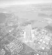
Shown here on the side is a 5-channel Landsat satellite photo of the mouth of the Taag in Portugal and the histogram, made with XITE, that belongs with it. The water causes the peak around gray level
10. The lowest gray level is 5 and the highest 243, but there are only a few pixels above 200. We could stretch the gray level linearly such that 5 falls on 0 and 200 is projected on 255.
An important aid in finding an appropriate gray level transformation is a histogram. A 2-D plot represents each
gray level on the x-axis and the number of pixels having that particular level given on the y-axis. Sometimes the values on the y-axis are shown as percentages of the quantity of pixels in the image.
Shown here on the side is a 5-channel Landsat satellite photo of the mouth of the Taag in Portugal and the histogram, made with XITE, that belongs with it. The water causes the peak around gray level
10. The lowest gray level is 5 and the highest 243, but there are only a few pixels above 200. We could stretch the gray level linearly such that 5 falls on 0 and 200 is projected on 255. The picture to the left shows a (part of) slide8 of the prostate CT images and the equalized histogram
version of it. The prostate is better visible there.
The picture to the left shows a (part of) slide8 of the prostate CT images and the equalized histogram
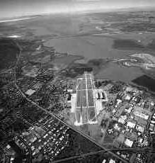
version of it. The prostate is better visible there. On the left is the previous Landsat image manipulated by the ideal LPF. The rings of
especially the rivers can clearly be seen.
On the left is the previous Landsat image manipulated by the ideal LPF. The rings of
especially the rivers can clearly be seen.