if f( x) ![]() T then pixel x belongs to the object or objects in the
image
T then pixel x belongs to the object or objects in the
image
< T then pixel x is a part of the background of the image
Contents:
During "thresholding" we use one or more threshold values. A pixel is given an area label depending on whether or not the intensity of the pixel satisfies the (non)equality relationships in which the threshold values occur. This is called the classifying of pixels, a simple example is:
if f( x)
T then pixel x belongs to the object or objects in the image
< T then pixel x is a part of the background of the image
This results in a binary image, but that alone is not yet segmentation. This must further be worked out by joining pixels together into one or more regions or areas.
 |
One way to determine a suitable threshold value T is to look at the histogram of the image. Ideally, the pixels of an object have a different intensity distribution than the pixels in the background. This is a global method, we do not look at the local environment of the pixel. Automatically separating the 2 peaks is a difficult problem when the histogram has many peaks lying close to each other or of very different in sizes. |
Some methods that are used are:
- to decrease statistical fluctuations, make the bins so large (by joining pixels) that on average many pixels lie in it.
-"smooth" the histogram, by comparing every bin with its neighbors and adjusting it to that (for example, fitting a parabola through 3 or 5 bins).
- search for the local maximum ( xi-1 < xi ![]() xi+1 ) and minimum
with overlapping sums of 2 sequential bins.
xi+1 ) and minimum
with overlapping sums of 2 sequential bins.
- fit 2 functions (for example Gaussian functions) on the histogram:
p(z) = ( P1 / ![]() (2
(2![]() )
)![]() 1 ) exp(- (z-
1 ) exp(- (z-![]() 1)2 / 2
1)2 / 2 ![]() 12) + (
P2 /
12) + (
P2 / ![]() (2
(2![]() )
)![]() 2 ) exp(- (z-
2 ) exp(- (z-![]() 2)2 / 2
2)2 / 2 ![]() 22) with P1+
P2= 1
22) with P1+
P2= 1
use a least squares method to determine the best parameters (in this case 5). If the histogram deviates from the function that must be fit, often a completely wrong result will come out.
A problem that often arises are weak variations in the gray levels of the background of an object, due to for example the lighting, see fig. 10.27. We would first use a high-pass filter to remove weak variations, possibly followed by noise removal.
 |
 |
We can also split the image up into rectangular sub images and make a histogram for each of those. For every histogram with a clear 2-peak structure, we can then determine the threshold. For sub images without a threshold determined in this manner, we take the (average of the) thresholds of the sub images near by. The total image is then thresholded by taking the thresholds determined for each particular sub image. |
|
|
|
Pixels on the edge of objects have a gray value between that of the object and that of the background. Making a gray level histogram of only pixels having a large edge value yields a peak, which is a good choice for the threshold. Vice versa, only the pixels with a small gradient can be taken or the pixels can be weighted with a factor 1/(1+G2). This results in sharper peaks and deeper valleys. One can also construct and analyze a 2-D histogram out of gray and edge values. |
Several thresholds can be derived from the histogram.
Sahoo, Soltani, Wong and Chen (CVGI 41, 233-260, 1988) give a classification and overview of thresholding methods and compare the results thereof on three images. A few methods with good results are described.
The method of Ostu is based on discriminant analysis. Thresholding can be seen as dividing an image in two classes and the ratios ![]() B2 /
B2 / ![]() T2
reflecting the distribution between the classes divided between the total distribution is minimized to t, the threshold:
T2
reflecting the distribution between the classes divided between the total distribution is minimized to t, the threshold:
T2 = i=0
g-1 (i-µT)2 pi with µT= i=0
0
µ0 = µt /T - µt) /
g: number of gray values; n: number of pixels; ni : number of pixels with gray level i
Kapur, Sahoo and Wong look at the gray level histogram as a source of l-symbols. Thresholding takes place if there is a division into two distributions. The total entropy (information contents) HB(t) +HT(t) is maximized:
HB(t) = - i=0
HT(t) = - i=t+1
Johannsen and Bille minimize the dependency (in information theory: meaning) between two distributions:
ln( i=0
ln( i=t
Kittler and Illingworth try to find a threshold such that an approximation to Gaussian function results in the left and right of the histogram.
In XITE 14 of these methods have been implemented. The found thresholds on the Landsat image are:
110 with OT (Otsu)
98 with KSW (Kapur, Sahoo and Wong)
114 with KI (Kittler and Illingworth)
These methods can be extended to cases where multiple thresholds must be determined.
With color (in general a vector value) images we can get intensity histograms for each different component, and also combinations thereof (for example R,G,B or I,H,S or Y,I,Q by color). The component with the best peak separation can then be chosen to yield the threshold for separating the object from the background. This method can be extended to a recursive segmentation algorithm, by doing the following for each region:
- calculate the histograms for each of the vector components.
- take the component with the best separation between two peaks and determine the threshold values to the left and to the right of the best peak. Divide the area into two parts (pixels inside and outside of that peak), according to those threshold values.
- every sub area can now have a noisy edge, improve that edge to make neat connected regions.
- repeat the previous steps for each sub area, until no histogram has a protruding peak.
 |
In (a) this method does not lead to a good segmentation, in contrary to that of (b). Using R+G and R-G components in (a) would have led to a good segmentation. For (a) we can also use the 2-dimensional histogram directly to look for peaks. Of course this is more difficult than looking for peaks in a 1-D histogram. |
The regions found using the previous methods are uniquely homogenous, resulting in a Boolean function H(R) with:
H( Rk ) = true for all regions k
H( RiRj ) = false for i
j combined regions
For example | f(x,y) - f(x',y')| < T , the regions pass the peak test.
 |
Horowitz and Pavlides (1974) organize the image pixels into a (pyramid) grid structure. Every region (except for 1 pixel areas) can be split up into 4 regions. Four regions on the correct position can be joined again to make 1 region. They used this structure in the following separate ∓ join algorithm working for every function H(): |
- begin with all the regions on a satisfactory level in the pyramid.
- if there is a Rk with H(Rk) = false, then divide the Rk into four even parts.
- if for the 4 sub regions, lying on the correct position, the following is true: H( Rk1![]() Rk2
Rk2 ![]() Rk3
Rk3 ![]() Rk4) = true, then join the 4 sub regions together to Rk.
Rk4) = true, then join the 4 sub regions together to Rk.
- repeat the last two steps until there is nothing left to divide or join
- finally join the regions together that do not fit into the pyramid structure neatly. If for neighboring Ri and Rj the following holds: H( Ri![]() Rj) = true , then join Ri and Rj.
Rj) = true , then join Ri and Rj.
Calculating H for all those regions can be time consuming. Sometimes H can be determined in such a manner that cases that are obviously not homogenous can be found quickly.
One starts with imagining each pixel as a region, afterwards those areas resembling each other are joined. Obviously there are many criteria possible to determine to which extent regions look similar.
|
|
|
With "Best Merge" the two regions most similar to each other are joined and this is continued iteratively (a clean sequential algorithm, and slow). In his thesis, Ron Schoenmakers created such an algorithm specially for satellite photos. First all the 4-connected pixels are joined into one region if they are exactly alike. |
|
|
|
Afterwards the two 4-connected areas with the smallest error criteria for merging are combined together to 1 region. This is repeated until the error criteria is larger than a certain threshold. The error criteria between two regions i and j was: Eij = |
In the image above each region has attained a gray value, different from its maximum 7 neighboring regions.
Other error criteria are possible as well, for example using the number of pixels per region or of the ![]() of
the gray values in regions. In his thesis Ron developed a parallel version of his method, for which also large images can be segmented in a decent amount of time. Using edge detection and edge
linking, a large image is first divided up into several regions. These can then be segmented independently using the best-merge.
of
the gray values in regions. In his thesis Ron developed a parallel version of his method, for which also large images can be segmented in a decent amount of time. Using edge detection and edge
linking, a large image is first divided up into several regions. These can then be segmented independently using the best-merge.
 |
Brice and Fennema (1970) use a "super-grid" for the representation of image and edge data. They use 3 criteria for the junction of regions, based on standards for edge strength and weakness: sij = | f(xi)-f( xj ) | ( crack edge) |
Sequentially the steps are:
- remove the edge between 4-connected xi and xj if wij(T1)=1.
- remove the boundary between Ri and Rj if:
W / min (pi, pj ) ![]() N1 with W=
N1 with W=![]() w'ij (T2) over the edge, pi is the circumference (in number of pixels) of
Ri
w'ij (T2) over the edge, pi is the circumference (in number of pixels) of
Ri
- remove the edge between Ri and Rj if: W (T3) ![]() N2
N2
The data structure mentioned above explicitly stores the edges but not the regions. Explicitly storing both the edges and the regions can be done with two graph structures:
- region adjacency graph: every node is a region, there is an arch between two nodes of which the regions touch each other.
- the dual graph of it: arches are edges, and nodes are locations where 3 regions touch each other.
A superficial region surrounds the original image. The necessary geometric information is stored in the nodes and arches.
Untill now the junction and splitting decisions were based on image data and on the weakest heuristical assumptions. Domain dependent knowledge (semantics) can also obviously be used for these decisions. A priori knowledge of certain regional interpretations (such as car, road, sky, etc. for a scene outside) can be related to measurable regional characteristics such as intensity, color, region size, edge length, etc.
Following the non-semantic criteria, Feldman and Yakimovsky also added semantic criteria:
1) combine regions i and j as long as they have a weak edge (threshold T1) in common.
2) combine regions i and j when:
(c1+aij) / (c2+aij)T2 for which c1 and c2 are constants and
aij = ((area1) +
(these first two steps are similar to what Brice and Fennema did)
3) let Bij be the edge between Ri and Rj. Evaluate every Bij with a Bayesic decision function which measures the probability with which Bij divides two regions with the same interpretation. Join i and j when the probability is high.
4) Evaluate the possible interpretations of each region Ri with a Bayesic decision function that measures with which likelihood Ri has been interpreted correctly. Assign the region with the highest value to its respective interpretation. Next improve the probability values of the neighbors of that region and repeat the assigning step until every region has attained an interpretation.
Steps 3) and 4) look for the interpretation of a given partition which maximizes the following evaluation function:
![]() ij P(Bij is an edge between X and Y|measurements on Bij ) P(Ri
is X|measurements on Ri ) P(Rj is Y|measurements on Rj )
ij P(Bij is an edge between X and Y|measurements on Bij ) P(Ri
is X|measurements on Ri ) P(Rj is Y|measurements on Rj )
 |
The measurements of the regions and edges can be given a numeric value and stored in a decision-tree (determined by correct segmentations of test images). |
The probability in step 3) is determined by: P = Pf / ( Pf + Pt ) (f=false, t=true) with
Pf = X
Pt = X,Y
and for step 4):
Confi = P(Ri is X1) / P(Ri is X2) (with X1 and X2 the most probable interpretations)
After region i has received the interpretation X1, its neighbors are adjusted as follows:
P(Rj is X) = P(Rj is X| measurements) P(Bij between regions X and X1)
We will only concentrate on a few topics from the large research area about moving images. From two pictures or a series of images taken quickly after each other, one can try to determine something about the motion in it (the movement of object or camera). All the points of an object make the same movement (translation and/or rotation). One can conclude information about objects and their motion from movement vectors.
The "optical flow" method assigns a 2-dimensional speed vector to each pixel in view. This vector shows the direction and speed with which the portrayed point has moved. No specific knowledge about the portrayed scene is used.
A time series of images is modeled as a function f(x,y,t), where it is assumed that f is "neat": the function is continuous and can be differentiated. Assume that during ![]() t the image moves over
t the image moves over ![]() x and
x and ![]() y:
y:
f(x,y,t) = f(x+x,y+
At small ![]() x,
x, ![]() y and
y and ![]() t and because f is "neat" we can write the Taylor expansion of f:
t and because f is "neat" we can write the Taylor expansion of f:
f(x+f/
The expansion part must thus be 0, and after neglecting e (the higher order terms) the following holds:
-
=
=f . u with
The gradient for each pixel can be determined from each image, and ![]() f/
f/![]() t from two consecutive images. The equation above can be restricted by u for every pixel to align in the
(u,v) space.
t from two consecutive images. The equation above can be restricted by u for every pixel to align in the
(u,v) space.
"Spatial redundancy" can be used to determine u because neighboring pixels often have almost the same speed. Horn and Schunck used this in the requirement that the derivative of the speed must be as small as possible. The above equation must also be complied with as much as possible. This leads to the minimization of the following function (Lagrange multiplier):
E(x,y) = (fxu + fyv + ft )2 +(ux2 + uy2 + vx2 + vy2 )
Here fx is a short notation for ![]() f/
f/![]() x, etc. Differentiate towards u (and the same for v) and equal it to 0:
x, etc. Differentiate towards u (and the same for v) and equal it to 0:
2 (fxu + fyv + ft) fx + 2
The last term is the Laplacian ![]() u, which we approximate by:
u, which we approximate by:
u(x,y) - 0.25 { u(x,y+1)+u(x,y-1)+u(x+1,y)+u(x-1,y) } or in other words:u = u - uav
Working this out even further results in:
u = uav - fx P/D with P = fx uav + fy vav + ft
v = vav - fy P/D D =
We solve these equations iteratively for u and v using the Gauss-Seidel method: make the first assumption of u(x,y) and v(x,y) and use it to calculate the left sides; the right sides will then
hopefully give a better approximation of u(x,y) and v(x,y). Repeat this several times, until the solution does not vary much anymore. The parameter ![]() , must be chosen appropriately. The first assumption u0 and v0 can be chosen as 0, or lying on the line given by the first
equation (for example both equal). In a series of images the end result of the first pair can be used as the initial value of the second pair.
, must be chosen appropriately. The first assumption u0 and v0 can be chosen as 0, or lying on the line given by the first
equation (for example both equal). In a series of images the end result of the first pair can be used as the initial value of the second pair.
 |
This method only works well for areas with a strong texture (local deviations in intensity) because then there is a decent gradient and the line limitations are bound to u. With small gradients the noise results in a relatively large error on the gradient, which continues to work on large errors on u. |
At edges (especially on both sides of a more or less uniform intensity) we can only determine the size of the displacement accurately in the direction of the gradient. This can be used to look at the movement of edges, from which the motion of objects can be determined.
 |
 |
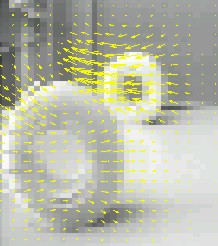 |
Two consecutive images and the calculated, smoothed optical flow (speed shown for each second pixel) by Alan Stocker. Click here for an animation of the optical flow.
 |
Results of Miki Elad. Row A gives the real optical flow from the synthetic series of images, row D gives the results of the Horn ∓Schunck algorithm. Rows B and C give the results of Miki Elad making use of the recursive approximated Kalman Filter algorithms. |
 |
When we move in an environment with static objects, then the visual world, as projected on the retina, seems to slide by. For a given direction of the linear movement and given the direction in
which to look, the world seems to come from one certain point in the retina, called the "focus of expansion" or FOE. This can be seen clearly by a video made with a quickly moving camera. For every
combination of movement and direction to look in, there is a unique FOE. When the movement takes place parallel to the retina, the FOE lies in infinity. |
Let all the objects move linearly with a speed of: (![]() x/
x/![]() t,
t,![]() y/
y/![]() t,
t,![]() z/
z/![]() t) = (u,v,w). In the image plane the movement of a point becomes:
t) = (u,v,w). In the image plane the movement of a point becomes:
(x0,y0,z0): ( xi, yi ) = ( (x0 + ut) / (z0 + wt) , (y0 +vt ) / (z0 + wt) )
From this we can derive xi = m yi + c where m and c are constants, independent of t. This movement thus follows a straight line that comes from ( taking t = - ![]() ) the point (u/w, v/w). This is independent of the position (x0,y0,z0) of the
point, every point on an object seems to come from (u/w, v/w), this is the FOE.
) the point (u/w, v/w). This is independent of the position (x0,y0,z0) of the
point, every point on an object seems to come from (u/w, v/w), this is the FOE.
Let D(t) be the distance from the FOE to the position of a point at time t and define V(t) = ![]() D(t)
/
D(t)
/ ![]() t, then one can derive: D(t) / V(t) = z(t) / w
t, then one can derive: D(t) / V(t) = z(t) / w
The right side is equal to the time that the object needs to reach the image plane. When the depth z of one point is known, then the depth of all the points can be calculated with the same w. Also the spatial coordinates of a point, with exception of a factor w, can be determined:
z(t) = w D(t) / V(t) , x(t) = xi(t) z(t) and y(t) = yi(t) z(t).
To determine the FOE on two images, it must be determined which pairs of points belong to each other: a portrayal of the same point on an object. This "match" problem is also well known as the "correspondence" problem. The images can be two consecutive images from a series and from the corresponding points the optical flow can be determined. It can also be done from a stereo image, the depth (the distance to the camera) of the objects can be determined from the pairs.
These types of algorithms are often composed of two steps. First candidate match points are found in each image independently. To do this one must choose image points that somehow deviate strongly from its environment. To do this, Moravec first defined the deviation for each pixel:
var(x,y) =
and IntOp(x,y) = min s,t var(s,t) with (s,t) in the environment of (x,y)
The IntOp values having the local maximum and those larger than a certain threshold value are chosen as candidate match points. This threshold value can be adjusted locally to yield a good distribution of candidates over the image.
For the second step, Barnard and Thompson use an iterative algorithm for the matching of candidate points. In each iteration n probabilities are assigned to each possible pair:
xi, (vij1,Pnij1), (vij2,Pnij2),... for every i in S1 and j in S2
making use of the maximal speed (or minimal depth): | vij | = | xj - xi | ![]() vmax
vmax
The assigned initial probabilities are:
P0ij = (1 + C wij) -1 with wij = D
In the following steps one makes use of the collective movement assumption (or about the same depth) to define the suitability of a certain match:
qn-1ij = ![]() k
k![]() l Pn-1kl with | xk - xi | <
l Pn-1kl with | xk - xi | < ![]() D (neighboring region) and |vkl - vij |<
D (neighboring region) and |vkl - vij |< ![]() V (almost
the same speed or depth)
V (almost
the same speed or depth)
And: P~nij = Pn-1ij ( A + B qn-1ij ) adjustment, Pnij = P~nij
/ ![]() k P~nik for normalization
k P~nik for normalization
The constants A,B,C ,![]() D and
D and ![]() V must be chosen suitably. After several steps, for each i in S1 the match with the largest Pnij is chosen. With this we can set preconditions, for
example that this one must be large enough and sufficiently larger than the following match. This also means that when two points are found that match with the same point in the second image, only
the best match has to be stored.
V must be chosen suitably. After several steps, for each i in S1 the match with the largest Pnij is chosen. With this we can set preconditions, for
example that this one must be large enough and sufficiently larger than the following match. This also means that when two points are found that match with the same point in the second image, only
the best match has to be stored.
 |
 |
 |
In motion analysis the FOEs which are found can be localized from the clustering of intersection points of lines through the found vij vectors. Found FOEs can be used again to find other matches or to remove incorrect matches. The found matches can also be used in the optical flow analysis, if the points have a static u and v. |
 |
Jain determined the FOE (when there was only one evident in the image) directly from the sets S1 and S2 candidate points without first matching them separately. For the set of points in the first image and corresponding points in the second image, the following equations hold for points O in the search space: L(OP'1) - L(OP1) <= L(P1P'1) |
with L(AB) the Euclidic distance between points A and B. The equals-sign is true when O=FOE. If
M(O) = ![]() L(OP'i) -
L(OP'i) - ![]() L(OPi) then M(O) is maximal when O=FOE.
L(OPi) then M(O) is maximal when O=FOE.
To calculate this function and to determine its maximum one does not have to match points. In practice the sets S1 and S2 will contain points of which the corresponding points are missing. This increases or decreases the function M(O) depending on the distance from O to the missing points (easily analyzed by regarding one additional, non-matching point). The function M(O) often behaves "neatly" and the maximum can be determined using simple gradient methods. When many corresponding points are missing, then the found FOE value will deviate from the real value. The found value can be used to match candidate points and for removing points which do not match or match or poorly. Finding the maximum of M(O) yields problems when the movement has a strong component parallel to the image plane, because then the maximum lies beyond the image; in the infinite when the movement is purely parallel.
Updated on March 4th 2003 by Theo Schouten.