Real-time
Linux (Xenomai)
Radboud University
Nijmegen
Exercise #10: Measuring Jitter
and Latency
Note: This
excercise is intended for a real hardware platform, although the
program for scheduling measurements could be tried first on VMware.
Introduction
In real-time programming one
usually has to guarantee that certain
deadlines are always met. Hence, predictability of timing is crucial.
In this exercise we investigate a few aspects of predictability by
measuring scheduling jitter and interrupt latency.
Objectives
The primary objectives of this
exercise are:
- To get experience with
timing measurements
- To investigate
predictability and timing characteristics of Xenomai by measure
scheduling jitter and interrupt latency.
Description
Terminology
We start with a definition of a number of terms, using a figure from
the presentation Real
Time
in Embedded Linux Systems by
Petazzoni & Opdenacker:
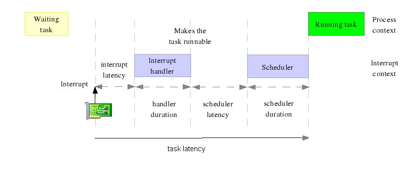
Interrupt latency: the time
between the occurrence of the
interrupt and the
start of the interrupt handler.
Scheduler
latency: the time
elapsed after completion of the handler and before execution the
scheduler .
Scheduling
latency, also
called
task
latency: the time between
the occurrence of the interrupt that
makes a sleeping task runnable again and the moment the task is resumed.
Scheduling jitter:
the
unwanted variation of the release times of a periodic task. It can be
characterized in various ways such as an interval around the desired
release time, a maximal deviation from the desired time point, or a
standard deviation from the mean value.
Pentium hardware and
performance
In the lab we use PCs with standard Pentium hardware which is optimized
for throughput, i.e., the number of instructions per time unit, at the
cost of predictable latency. This means that we rather have a
high
average speed of instructions than a guaranteed low execution time of a
specific
instruction. The optimizations used by Pentium hardware makes most
instructions executed very fast. Occasionally, however, a
single instruction might take much longer to execute than it
would do without optimization. This is problematic for real-time
systems that need guaranteed hard real-time
deadlines.
Unpredictability
Execution time
We list a number a number of reasons that contribute to the
unpredictability of the execution time of instructions:
- Optimization techniques used
in CPU design :
- Pipelining
is used in modern Intel processors to run a set of
instructions in parallel.
- Branch
prediction
When trying to execute
more instructions in parallel, there
is a problem with branch instructions. Then not all information might
be available yet to decide which instructions to execute. Instead of
waiting until this info is available, the CPU does ad
educated guess (prediction) of the result of the branch instruction.
After that it already starts executing independent instructions from
that branch in parallel. If the guess was wrong, the results
are thrown away and execution continues in the other branch. If the
guess is right, throughput has been increased.
- Out-of-order
execution
When a certain instruction has to wait for available data, subsequent
instructions are already executed (out-of-order) and the results are
re-ordered later to reconstruct the logical order.
These techniques are rather complex and they make it is difficult to
predict exactly
when an single instruction will executed.
- CPU
cache
Caches are used because of price-performance optimizations:
- Cache memory is 10 times
faster than RAM memory
- RAM is much cheaper than
cache memory
- Often a relatively small
part of memory is used most
frequently, so by using a small piece of fast memory (the cache) access
to slower RAM is occurs infrequently and the machine becomes faster at
relatively low costs. But it increases unpredictability:
instructions are fast if the data is in the cache, but become slower
if data is not in cache (a so-called "cache miss")
and (1)
some space in the cache has to be made, and (2) data has to be accessed
from slower RAM and stored into cache.
- Address
Translation Cache (ATC) is used
by the memory management unit
to get a quick access to the address translating table in memory.
A cache miss, however, leads to additional time.
- Paging
implements virtual memory: it uses RAM as a cache for hard disk
memory. Here a cache miss is called a "page fault" and also leads to
additional time.
- Direct
Memory Access (DMA) is a
hardware mechanism which allows data
transfer in parallel with other instructions executed by the CPU.
Having a DMA channel leads to less CPU overhead for data transfer, but
it may occupy the entire memory bus
asynchronously from what the CPU is doing. Hence a process that needs
access
to RAM might have to wait for a long time for a DMA
operation to complete.
- Interrupts
An example of the worst case execution scenario of an instruction :
what
happens
time cost in nanoseconds
-------------------------------------------------------------------------
-
execution time
instruction
1 ns
-
instruction cache
miss
50 ns
-
instruction ATC
miss
500 ns
- data
cache
miss
1 000 ns
- paging
needed for instruction
and data 90 000 000 ns
- many
interrupts during
execution
100 000 ns
- one big
DMA
10 000 000 ns
-------------------------------------------------------------------------
total : 100 101 551 ms
Hence, the execution of an instruction which basically costs a few nano
seconds might take more than 100 milli seconds.
Interrupt latency
Besides the causes mention above, there a few additional factors that
contribute to the unpredictability of interrupt latency.:
- The CPU has to finish the
current instruction (some instructions take 10
TSC clock ticks)
- Context saving time
- Time to switching to ISR
(read IRQ table, setup ISR stack)
- Interrupt masking: when
interrupts were disabled at the occurrence of an interrupt, it has to
wait until they are enabled
again
- Interrupt priority: the
servicing of low priority interrupts
is delayed when a higher priority interrupt is being serviced
Scheduling
latency
For scheduling latency the same factors apply as for interrupt
latencies. However in this case extra latency can be caused that the
schedular has to wait for the Linux kernel to complete some other tasks
before it can execute.
When we periodically schedule a task, each cycle of the task starts
late caused by the scheduling latency. Some part of the scheduling
latency is sporadic, but other parts like e.g. "context saving" time is
reocccuring for each cycle. Thus there is some fixed part of the
scheduling latency reoccuring for each cycle. This means that when we
take the difference between two adjacent cycle times, we remove this
fixed part! Thus the latency between relative scheduling times of the
periodic task are smaller. Hence the variation of the scheduling
latency is smaller!
Load on a Linux system
To investigate how the load of a system affects jitter and latency, we
will put some load on the system when performing measurements. We
discuss a number of ways to monitor and to add various types of load on
a Linux system.
I/O network load
I/O disk load
- Monitor tool:
- in terminal
: iotop
(needs IO_ACCOUNTING option in kernel)
- in gui: gnome system
monitor
- Load tools
using dd:
- big write, no read : dd
if=/dev/zero
of=/tmp/bigfile
- big read, no
write : dd if=/dev/hda1 of=/dev/null
bs=1000k
==> watch out when using /dev/hda1 : a typo can delete
your
harddisk!!!
- big read and write : dd
if=/dev/hda1 of=/tmp/bigfile
bs=1000k
==> watch out when using /dev/hda1 : a typo can delete
your
harddisk!!!
using 'ls -lR':
- while true; do ls -lR
/ > /tmp/list ; done
&> /dev/null
CPU load
- Monitor tool: top, htop
- Load tools :
- CPU
burn-in:
The program heats up any x86
CPU to the
maximum possible operating temperature that is achievable by using
ordinary software.
- Hackbench:
The hackbench test is a
benchmark for
measuring the performance, overhead, and scalability of the Linux
scheduler.
- while true; do cat
/proc/interrupts >/dev/null ; done
=> high CPU
load in kernel mode
- while true; do (( 3+4 ))
>/dev/null ; done
=> high CPU load in
user mode
Memory load- swapping
- monitor tool:
top, htop
- load tools:
use memoryload.c :
#include <stdlib.h>
main() {
 while (1) {
 malloc(10240);
 }
}
Exercises
Exercise 10a.
Write a program to collect
data about the real periodic
scheduling of a task and plot this data.
Approach:
- Write a periodic real-time
task which is scheduled every 100
microseconds and which executes 10 000 times.
- At the beginning of each run
of the task, read the current time with "rt_timer_read" (which returns
a value of type RTIME) and store this in a global array.
- After reading all values, compute the difference between each
pair of successive times (which should be close to 100 000 ns) and
store this in another array.
Write this last array to a
comma separated file (.csv) of the form:
0,value[0]
1,value[1]
2,value[2]
....
For instance, by
write_RTIMES("time_diff.csv",nsamples,time_diff);
void write_RTIMES(char * filename, unsigned int number_of_values,
                  RTIME *time_values){
         unsigned int n=0;
         FILE *file;
         file = fopen(filename,"w");
         while (n<number_of_values) {
              fprintf(file,"%u,%llu\n",n,time_values[n]);
              n++;
         }
         fclose(file);
 }
- Open this .csv file in a
spreadsheet (e.g., in Excel) and plot the data in graphic
showing the measured value in the y-axis and the number of the
measurement in the x-axis. [The comma in the .csv file should lead to
two columns; if
this does not work - maybe because of language settings - try replacing
the comman by ";".]
Try the measurments first in VMware and next on a Linux PC. Describe
the results.
Exercise 10b.
Use the spreadsheet to calculate the average value of the measured
periods, the maximal and minimal deviation from the desired period (100
000), and the standard deviation of the timing differences.
Exercise 10c.
Use the following combined.sh
script
to put Linux under a big load:
    #!/bin/sh
    ping -f localhost -s 65000  >/dev/null   &  # network load
    while true; do cat /proc/interrupts >/dev/null ; done &  # cpu load
    while true; do ls -lR /  > /tmp/list ; done  &> /dev/null  # disk load
- Look at the contents of this shell script (e.g. by "cat combined.sh"), run the script
and monitor the load increase.
- An option is to run the script in one console (./combined.sh) and to switch to
another console with Ctrl-Alt-Fx
to perform some monitoring. To stop the load, return to first console
and stop the script by Ctrl-C.
- An alternative is to start the script on the background
(./combined.sh &), perform monitoring on the same console, look at
the running processes with "ps -a"
and their PID, and stop the load processes explicitly with "kill -9 <pid>".
- Note that not all monitoring tools are available under VMware.
- Start the shell script and next rerun the jitter measurements
concurrently with the additional load. (Stop the load processes
afterwards.)
- Describe and analyze the results.
Exercise 10d.
Use the special parallel port cable to connect two PCs running
Xenomai to each other. This special cable connects in both ways the
data line D0 from one machine to the interrupt line S6 of the other
machine. Now write a program to measure the interrupt latency of a PC
as follows:
- On both PC 1 and PC 2 keep
data line D0 high.
- On PC 1 measure the
time t1 and generate an interrupt on PC2
by pulling data line D0 low and then high again.
- On PC 2 write an interrupt
handler for the parallel port which
generates an interrupt on PC1 by pulling data line D0 low and
then
high again.
- On PC 1 write an interrupt
handler for the parallel port which
measures the current time t2.
Repeat this measurement 10.000 times every 100us, and compute in
each case the interrupt latency.
Similar to the exercise on scheduling jitter, write the results to a
file, plot the measured latencies in a graph, and calculate average
latency and the standard deviation.
Last Updated: 26 September
2008 (Jozef Hooman)
Created by: Harco Kuppens
h.kuppens@cs.ru.nl