 Both a CCD and a normal camera record a 2-dimensional digital intensity image. Throughout this
course we will concentrate on methods which process these types of images. Most of the methods are applicable to many ultrasound, 2-D CT and depth images.
Both a CCD and a normal camera record a 2-dimensional digital intensity image. Throughout this
course we will concentrate on methods which process these types of images. Most of the methods are applicable to many ultrasound, 2-D CT and depth images.Contents:
Both a CCD and a normal camera record a 2-dimensional digital intensity image. Throughout this
course we will concentrate on methods which process these types of images. Most of the methods are applicable to many ultrasound, 2-D CT and depth images.
The 3-D CT and MRI images can be edited by simply extending the 2-D algorithms; for example, replacing a pixel value by the average of its 9 2-D neighbors will become a replacement by the average of its 27 3-D neighbors.
With Shape from Shading one tries to determine the form or position of objects by examining the reflection of light from a more or less known light source or the shadow that is created from it.
With Inverse Perspective one tries to determine the distance to an object or the orientation of it by using the perspective transformation of the camera lens. An object far away is projected smaller than an object close by. A circle viewed at an angle is projected as an ellipse.
Stereo Matching uses two images from cameras located close to each other. The slightly deviating positions of the object in the stereo images can be used to calculate the distance to the
object.
Movement of objects can be determined from a series of intensity and depth images.
Both the TV video camera and the CCD camera have a lens system which projects reflected light in a 3-D scene onto an image plane. The less popular TV video or vidicon camera uses a photo conducting plate on which a charge is created that is proportional to the amount of light striking it. Consequently an electron bundle is used to read out the charge. A CCD (Charge Coupled Device) is a chip that contains a matrix of capacitors, which record the charge when light creates electron hole pairs. By applying a suitable voltage to the contact points, shifting the charge from one capacitor to another, making it possible to determine the charge which was created by the light.
 |
In a full frame CCF, the shutter of the lens is closed after exposure to light and the image is repeatedly shifted one row downwards. Every row is placed in a serial register so that the charge of each independent pixel can be determined. A frame first transfers the entire image to a storage matrix which is in turn read out serially, while the next image sensing can start. |
An "interline transfer CCD" shifts each column into a neighboring column which is not light sensitive, and then read out. This happens very quickly so that the use of a shutter is not necessary; however, less than half of the incoming light is used; a geometric pixel only registers the light in its left half. In other CCD types some of the geometric pixels are not used due to the boundaries between the pixels and the metal contacts.
A CCD yields less noise in its images than a TV camera. This can be limited even more by cooling the chip, sometimes as low as the temperature of liquid helium. The geometric distortion is also smaller due to the lack of an electron bundle which has to be shifted over the entire image.
 |
For acquiring a color image, one uses a different CCD chip with color filters in front of it for each color is used. The light is divided evenly over the three CCDs. The pixels of each CCD are
made susceptible to one of the red, green or blue components of light by placing a filter in front of it. To do this, one uses a Bayer pattern to calculate one RGB pixel out of a block of 4 pixels,
or four RGB pixels using interpolation. The color green is measured more frequently because it yields the best results. |
The analog output of the serial register, the video signal, uses an Analog to Digital Converter to convert the output to a digital signal; a measurement for the amount of light that has fallen on the pixel. This happens frequently in a frame grabber, which additionally uses pixel shift signals that are generated by the electronics in the CCD chip. A frame grabber often contains memory for storing one or more images and is connected to a standard computer bus (PCI, VME, SBUS, etc.). Sometimes it contains a microprocessor, a DSP or special hardware for quick processing of the acquired images.
 |
 A CAT (Computer Aided Tomograghy) or CT (Computed Tomography) scan uses an x-ray source to measure the
non-translucency of the slice of an object. Numerous one-dimensional projections are taken under different angles. From those projections a 2-D intensity distribution is calculated throughout the
slice. This results in an image that gives an impression about the inside of an object. The newest types of Spiral CT for medical applications rotate the x-ray source around the patient while the
patient is slowly moved through the machine. In 30 seconds, while the patient is holding his breath, a 3-D image of the chest is recorded. A CAT (Computer Aided Tomograghy) or CT (Computed Tomography) scan uses an x-ray source to measure the
non-translucency of the slice of an object. Numerous one-dimensional projections are taken under different angles. From those projections a 2-D intensity distribution is calculated throughout the
slice. This results in an image that gives an impression about the inside of an object. The newest types of Spiral CT for medical applications rotate the x-ray source around the patient while the
patient is slowly moved through the machine. In 30 seconds, while the patient is holding his breath, a 3-D image of the chest is recorded. |
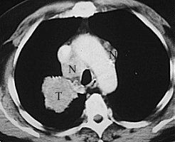 |
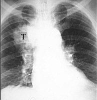 The photo on the right is a regular x-ray photo of a chest with a tumor (T). The photo on the left is a CT
scan straight through the tumor, which can now be seen clearly, as well as the metastases (N) next to it. The photo on the right is a regular x-ray photo of a chest with a tumor (T). The photo on the left is a CT
scan straight through the tumor, which can now be seen clearly, as well as the metastases (N) next to it. |
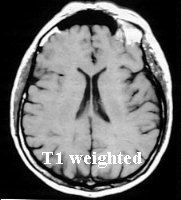
MRI (Magnetic Resonance Imaging) uses NMR (Nuclear Magnetic Resonance) to reconstruct a 3-D image. The patient lies in a strong magnetic field (1.5T or 15000 Gauss; to put that into perspective, the earth's magnetic field is about 0,6 Gauss) so that the spin of the freely or bonded protons of the tissue point in the direction of the field. Then, an electromagnetic pulse with a certain radio frequency is beamed in which disrupts the direction of the spin. Two types of relaxation processes, spin-lattice or T1, and spin-spin or T2, are responsible for the fact that the protons point in the direction of the field again while broadcasting the electromagnetic radiation. For a large number of pulses this radiation is collected through an antenna, used by a computer program to calculate the 3D images. These intersections (often transversal, coronal or {VERTAAL saggitaal , sagital}) can be shown on a monitor.
 |
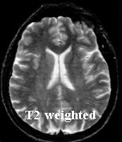 |
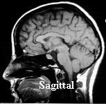 Two transversal and one {VERTAAL sagital} image. Two transversal and one {VERTAAL sagital} image.The CT and MRI images here have been borrowed from Imaging Tutorial |
 |
A T1 weighed imaged exemplifies the difference in T1 relaxation between tissues. Because the water shown here is black, the anatomic details are well visible. In a T2 weighed image water is shown as white. Because pathological processes (tumors, injuries, cerebral bleeding, etc.) are often recognized by the forming of water, a T2 image is appropriate for distinguishing between normal and abnormal tissue. A slice through a prostate gland (Henkjan Huisman, Radiology AZN), click here for a series of 11 slices. Other atom nuclei such as 13C and 31P characterize the NMR effect as well. With NMR-Spectroscopy one examines the received electromagnetic radiation more accurately because the received frequency, measured in ppm (partspermillion), depends slightly on the position of the atomic nucleus in the molecule. From the resulting spectrum one can determine the presence and concentration of certain molecules. |
The old photographic film is still used frequently to sense and acquire an image; it has a high resolution and is easily viewed with the naked eye. A photo or text on paper is transposed to a digital image by a scanner. It uses a streak of light, generated by a row of LEDs (Light Emitting Diodes), projected on the and measures the reflected light by a row of CCD pixels or other light sensitive cells such as photodiodes. Afterwards, the light streak or the paper is moved to measure the next row.
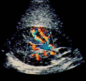 |
An ultrasound camera is used to record the reflection of a high frequency (1-15MHz) sound bundle, which can be generated and collected by a transducer. One can determine the reflection (amount of reflected sound), depth (from the time taken to receive a reflection) and movement (by Doppler effect) properties of the objects. This is frequently used for medical applications and inspection of the inside of a fabricated product (such as a car engine). The included image (The Burwin Institute) is of a healthy kidney; the color shows the speed of blood moving through the veins. For more information about ultrasound see Medical Ultrasound Imaging WWW Directory. Sonar works much the same. |
The 'structured light' method projects structured light on a 3-D scene, for example (multiple) points, lines, a grid or light with a consequent intensity. The form and depth of the objects can easily be derived from the measured reflection. With the help of imaging technology, appropriate control over the welding apparatus, a well-chosen wavelength of structured light and an appropriate light sensitivity of the sensor, one can avoid that the light of the welding process results in image distortion. (Images from Weld Seam Determination Using Structured Light )
 |
 |
 |
A 'spot ranger' projects a small laser, infrared or ultrasound spot on a scene. From the direction of the reflected bundle (triangle measurement, here on the side) or from the time to reflection
(see above) the distance to the object can be calculated. The distance to the object must repeatedly be determined for each direction (pixel). Determining the complete image is a lengthy process. One
usually first uses a regular picture to determine the object to which you want to know the distance to. We know two methods for determining the distance when focusing a camera; an active and a passive method. The active method uses an infrared bundle. The amount of reflected light which is received is proportional to the distance to the object. Then the aid of a motor, the lens is the placed in the appropriate position. |
 |
 |
With the passive method, a CCD camera lens is moved until (the center of) the acquired image is as sharp as possible. The average difference between the pixels and their neighboring pixels is used to determine the how sharp the image is. |
During imaging, often mathematical models of images and image creation are used. For example, one can use the following model to determine deviations in the image due to the lens, to measure its parameters for a specific system and then correct the image for those deviations.
An image function is a mathematical representation of an image, for example: f(x) = f(x,y) the light intensity or energy on position x. One can write: f(x) =
i(x).r(x) with i(x) the illumination and r(x) the reflection. Both are limited: 0 <= i(x) <= ![]() and 0 <= r(x) <= 1, correspond to the total absorption and total reflection. Often only r(x) is of importance, but
with structured light and shape from shading i(x) plays an important role. In black and white images, f(x) is a scalar value; in multi-spectral images f(x)
is a vector value. Color images have f 3 dimensions: f(x) = { fred(x), fgreen(x), fblue(x)}. However, remote sensing images
are taken from satellite or airplane, resulting in an image which can be anywhere from 30 to 256 dimensions. For 3-D images one uses x= {x,y,x}, and for a time series of images:
f(x,t).
and 0 <= r(x) <= 1, correspond to the total absorption and total reflection. Often only r(x) is of importance, but
with structured light and shape from shading i(x) plays an important role. In black and white images, f(x) is a scalar value; in multi-spectral images f(x)
is a vector value. Color images have f 3 dimensions: f(x) = { fred(x), fgreen(x), fblue(x)}. However, remote sensing images
are taken from satellite or airplane, resulting in an image which can be anywhere from 30 to 256 dimensions. For 3-D images one uses x= {x,y,x}, and for a time series of images:
f(x,t).
 |
A digitizing model then describes the digitalization of the space and time coordinates, called sampling, and that of the intensity values, named quantization. CCD cameras and scanners often use squares to do the sampling; the incoming radiation is then integrated over the area or part of it. For images which must be shown on a television, rectangles with sides in the ratio 4:3(the aspect ratio) or 16:9 for the newest wide screen TV standard. Other formats are also used for experimental CCD cameras such as hexagonal pixels. These have the advantage that a pixel has only one type of neighboring pixel. |
 |
When choosing a zoom lens camera system, make sure that the resolution is high enough so that the smallest detail has a surface area of at least one pixel. How many pixels are needed depends on
what needs to be measured and with which accuracy. The higher the resolution, the more disk space is required for its storage. The calculation time for algorithms also grows, sometimes as n.ln(n),
n2 or n3, n being the amount of pixels. |
 |
That is why resolution pyramids are used: for example from a 512*512 acquired image, we first calculate the 256*256, 128*128, 64*64, etc. images. Finding objects can occur in the 64*64 image. Determining the surface of an object is therefore more precise in the 512*512 image. Of course, the gain in time must be weighed up against the time needed to build the pyramid as well as the extra memory needed to store the images. However, the amount of pixels in the extra images will never be more than the amount of pixels in the original image (see chapter 7.1.1). The amount of bytes needed to store intermediate data, such as the edges of the objects, could be less. |
 |
Energy falling on the sensitive surface of a pixel becomes quantised in several steps: in machine vision 1 bit is sometimes used for binary images, but usually 8 bits, so 256 steps or gray levels, are used. Lately people tend to use more bits; 10, 12 or 16 is not irregular anymore. With CCD cameras and scanners people try to make the relationship between energy and gray level as linear as possible. |
 |
The effect of different ranges of gray levels can be seen in [fig. 2.21]. The amount of bits used has an influence on the storage of the image. If this takes place elsewhere than in a byte or a short integer (16 bits), then unpacking will be mandatory for editing on a regular computer, which is undesirable. |
These describe the geometric relationships between the coordinates of a point in a 3-D space and the coordinates of its projection.
 |
In general X = {X,Y,Z}T and x = {x,y,z}T do not coincide, T represents a transposition and turns a row vector into a column vector. We must first find the transformation matrix that projects X onto X' and coincides with x: X'h = M Xh, where M is a 4 by 4 matrix and Xh= {X,Y,Z,1}T is the homogenous version of X. Paragraph 2.5.1 shows how M can be built up from translation, rotation and scaling matrixes, and 2.5.3 shows how M can be calculated from the position and orientation of the moving camera.
 In general, additional equations can be derived from a point X in a random world
coordinate system and its projection x = u/w and y = v/w in the resulting image. Each measurement (x,y) of a known point X results in 2 equations with 12 unknowns. Six measurements, with no
two points X on one line through the lens center, should be sufficient to determine matrix A. In practice we need many more points and need to use a numeric method to determine the optimal
result for A from the derived equations. This process is called the calibration of the camera system. That this is laborious is due to the fact that distortions in the lens system are taken into A,
which can't be dealt with by such a simple matrix. So lens distortions must be corrected separately, for example x' = c0 + c1x + c2y + c3x2
+c4xy +c5y2 +... sometimes until 5th order formulas that are derived from the type of lens system and the manner in which they are mounted. The parameters
c only have to be calculated once after the camera's assemblage. This is done by measuring a large amount of points on the known grid [fig. 5.34]. The matrix A must be recalculated after every
position adjustment of the camera, using the values x' and y' after correction for lens distortion.
In general, additional equations can be derived from a point X in a random world
coordinate system and its projection x = u/w and y = v/w in the resulting image. Each measurement (x,y) of a known point X results in 2 equations with 12 unknowns. Six measurements, with no
two points X on one line through the lens center, should be sufficient to determine matrix A. In practice we need many more points and need to use a numeric method to determine the optimal
result for A from the derived equations. This process is called the calibration of the camera system. That this is laborious is due to the fact that distortions in the lens system are taken into A,
which can't be dealt with by such a simple matrix. So lens distortions must be corrected separately, for example x' = c0 + c1x + c2y + c3x2
+c4xy +c5y2 +... sometimes until 5th order formulas that are derived from the type of lens system and the manner in which they are mounted. The parameters
c only have to be calculated once after the camera's assemblage. This is done by measuring a large amount of points on the known grid [fig. 5.34]. The matrix A must be recalculated after every
position adjustment of the camera, using the values x' and y' after correction for lens distortion.
For a stereo recording the simplest solution is using 2 cameras whose axis are parallel to each other but with a slight deviation B in the x direction (or in the y direction). A point X is
then projected in both cameras at a slightly different x value. The shift (x2-x1) can be calculated in Z. To derive the given formula look at the triangles that have been formed
(be careful: coordinates can be negative, the length of a line can't). Of course it must be known that the points x2 and x1 have been derived from one point X: the
correspondation problem. This problem especially plays a role with serial images, where the camera and/or object has been moved. The absolute (in pixels) measurement error on
(x2-x1) depends solely on the resolution of the spatial sampling, not on the size of (x2-x1). At a small Z, (x2-x1) is larger than at
a large Z, the absolute error on Z becomes larger while Z becomes larger: ![]() Z ~ ((Z-
Z ~ ((Z-![]() )2 / B )
)2 / B ) ![]() x. At larger B values, Z can be determined more precisely, but the correspondation problem becomes more difficult and the two images will show less overlap with each other. By
placing the cameras at a certain angle instead of parallel increases the overlap but makes the calculation of Z more difficult.
x. At larger B values, Z can be determined more precisely, but the correspondation problem becomes more difficult and the two images will show less overlap with each other. By
placing the cameras at a certain angle instead of parallel increases the overlap but makes the calculation of Z more difficult.
Radiometric models describe how light emitted by an object in a scene reflects or falls on the image plane.
What does this mean? The energy E of a pixel (and thus its gray level) is proportional to L, the emission of energy from the object. It is also proportional to D2, the surface area of the
lens, usually equal to the opening of the diaphragm in front of the lens. And also proportional to cos4![]() , with
, with ![]() the angle at which the camera sees the object. A flat object emits light in
all directions evenly, however, placed at a distance fo right in front of the lens shall not show the same gray level for each pixel. The gray level decreases the closer the pixel lies to
the middle.
the angle at which the camera sees the object. A flat object emits light in
all directions evenly, however, placed at a distance fo right in front of the lens shall not show the same gray level for each pixel. The gray level decreases the closer the pixel lies to
the middle.
The human eye has the following sensitivity to light:
 |
Sensitivity of the 3 types of cones and rods in the eye. |
The blue cones are the most sensitive, but they are scarce; out of all the cones, 65% is red, 33% is green and only 2% is blue sensitive.
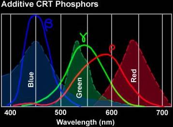
 R,G,B are the primary colors. Additive mixing yields more colors, such as a color monitor showing the secondary colors
Cyan (G+B), Magenta or purple(R+B) and Yellow (R+G). The primary spectrum emitted by a monitor does not exactly coincide with the sensitivity of the eye (see here on the side). It is often possible
to correct this to create a natural image. R,G,B are the primary colors. Additive mixing yields more colors, such as a color monitor showing the secondary colors
Cyan (G+B), Magenta or purple(R+B) and Yellow (R+G). The primary spectrum emitted by a monitor does not exactly coincide with the sensitivity of the eye (see here on the side). It is often possible
to correct this to create a natural image. When light falls on a color print on paper, the material absorbs some wavelengths and reflects others. Here C,M and Y are
primary colors. When light falls on a color print on paper, the material absorbs some wavelengths and reflects others. Here C,M and Y are
primary colors. |
 |
 |
The RGB color model, appropriate for working with color monitors and most cameras and scanners, represent the R,G and B as values between 0 and 1. In the computer these become positive numbers ranging from 0 to the maximum value, usually 255, 1 byte per color. A color is represented as a point in a 3-D RGB cube. Here R is normalized to 700 nm, G to 546.1 nm and B to 435.8 nm. However, it isn't possible to show all the existing colors with this model, see fig 6.6. |
 |
If a display card of 3 bytes per pixel is used, we call it a true color display with a maximum of 2563 or about 16 million colors per picture. Because this requires a lot of memory, usually a pseudo color display is used, with 1 byte per pixel, a maximum of 256 colors per image. A color lookup table (CLUT) makes it possible to choose any one of the 16 million colors for each of the 256 colors in an image. |
With the CMY models a color {C= 1-R, M= 1-G, Y= 1-B} can yet again be represented with a 3-D cube. The model is appropriate for color printers and color printing processes. A problem here is that
the color black can't precisely be made. The top layer of the ink always reflects some light, making the black look brown. For nice prints using black ink one can use the CMYK model (K stands for the
color Black, B has already been used for blue). This model can be calculated from the CMY as follows: K:= min(C,M,Y), C:=C-K, M:=M-K, Y:=Y-K.
For color TV broadcasting other models are used, such as the YIQ model or the YUV model, sometimes called the YCbCr model. Old black and white televisions could receive the broadcasts but only used the Y signal. The color components could be broadcasted at a lower resolution (in PAL 5 MHz for Y and 1,3 MHz for U and V) and still give a satisfactory television image.
The previously described models were fairly hardware oriented. There are also models that concentrate on the manner in which people describe colors. Here terms such as Hue (the average color), Saturation (the purity of a color or the lack of white) and Intensity or Brightness (intensity or amount of light).
With square or rectangular pixels, each pixel p with 4 neighboring pixels shares an edge with each of its neighbors, the so called 4-neighbours, and make up the set N4(p). With four other neighbors the pixel only shares a vertex, the d-neighbors in the set Nd(p). Therefore there are eight neighbors with which the pixel shares an edge or a vertex, the 8-neighbours in the set N8(p).
Pixels p and q with gray levels chosen from a set V, e.g. V={1} for binary images or V={100...150} for byte images, are 4-connected if q ![]() N4(p); and 8-connected if q
N4(p); and 8-connected if q![]() N8(p) and m-connected
if q
N8(p) and m-connected
if q![]() N4(p) or if q
N4(p) or if q![]() Nd(p) en N4(p)
Nd(p) en N4(p) ![]() N4(q) = Ø. This m-connectiveness
eliminates ambiguities:
N4(q) = Ø. This m-connectiveness
eliminates ambiguities:
 |
Subsets S1 and S2 of an image are (4, 8 or m) connected if there is a pixel in S1 that is (4, 8 or m) connected with a pixel in S2. A (4, 8 or m) path from p to q is a row of pixels with p the first and q the last where each consecutive pair of (4, 8 or m) pixels is connected. Two pixels composed from the subset S are connected if a path exists between them that is only composed of pixels from S. For each pixel p from the subset S (called the set S1) made up of pixels from S connected to p is called a connected component of S. |
Finding and marking the 4-connected regions in a binary image is sometimes called the connected component labeling or blob coloring. Given a binary image with 4-connected "blobs" of ones on top of a background of zeros, we try to label or color each blob uniquely. This can be done using the following algorithm.
| f(xu) | f(xl) | do: |
| 1 | 0 | color(xc) := color(xu) |
| 0 | 1 | color(xc) := color(xl) |
| 0 | 0 | color(xc) := k ; k := k+1 |
| 1 | 1 | color(xc) := color(xu) or color(xl) and store in a list: color(xu) == color(xl) |
The image is analyzed as a grid, from left to right and from top to bottom. For each pixel xc we look at the pixel to its left xl and the pixel above it xu, which
have both previously been visited. If f(xc) = 1 , so that xc belongs to some surface, then follow the instructions in the table.
After this scan every pixel has its own color value. Some color values are equivalent and therefore must all be replaced with one and the same color value. For this the image must once again be analyzed, unless we had kept a list with which pixels have which color. The algorithm above only shows the essence of the idea; the initialization, where and how to save the color and what to do with the pixels that don't have a left or an upper neighbor is not explained. That is up to you to decide. The algorithm can easily be adjusted to find 8-connected regions.
D is the distance function or measurement between points in a n-dimensional space. For all the points p, q and r the following holds: D(p,q) ![]() 0 ; D(p,q) = 0 iff p=q ; D(p,q) = D(q,p); D(p,q) + D(q,r)
0 ; D(p,q) = 0 iff p=q ; D(p,q) = D(q,p); D(p,q) + D(q,r) ![]() D(p,r). For the measurement between 2 points (x1,y1) en (x2,y2) in 2-D images we have the following example:
D(p,r). For the measurement between 2 points (x1,y1) en (x2,y2) in 2-D images we have the following example:
| Euclides | ( (x1-x2)2+(y1-y2)2 )1/2 | |
| perpendicular | | x1-x2 | + | y1-y2| | D4 or city-block distance |
| maximum | max { x1-x2 , y1-y2} | D8 or chessboard distance |
Arithmetic operations can be applied on pixels p and q on the same position in 2 images of the same size; examples are: addition, subtraction, multiplication and division of pixel values. A practical application of + and / is the averaging of images to diminish noise. Subtraction is used for Digital Subtraction Angiography (DSA) in medical applications where sensing recordings are made before and after the injection of a contrasting liquid in the veins. Subtraction of the images will give a good impression of the circulation in the veins or possible obstruction thereof.
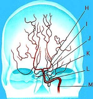 |
 Click here for a series of DSA images (animated GIF) see Angiography for more information. |
Logical operations (AND, OR, XOR, NOT) are also applied to binary images. If the operations are not executed on the entire image but only a part of it, they are called ROI (Regions of Interest).
Arithmetic and logical operations can also be executed within one image. With a convulsionary operation the pixel receives a new value depending on its old value and that of its neighboring pixels:
 W is called a mask, template, window or filter. A convolution is an example of a parallel operation: it
is conceptually executed on all the pixels in the image simultaneously. Parallel operations are easy to implement in specific hardware (ideally 1 CPU per pixel, which has access to the 8 or more
neighboring pixels) or in special "systolic" hardware. Modern "frame grabbers" often have enough memory for two images with a shift/ALU hardware [table 2.3] with which the convolution operation can
be done in 9 "frame times" (1/30 or 1/25 s). Contrary to serial operations: there the pixels are visited consequetively and the newly calculated value of a pixel is used to calculate the next pixels
(an example of this is the blob color algorithm). Such a serial algorithm is often faster to implement on a general purpose computer than a parallel algorithm.
W is called a mask, template, window or filter. A convolution is an example of a parallel operation: it
is conceptually executed on all the pixels in the image simultaneously. Parallel operations are easy to implement in specific hardware (ideally 1 CPU per pixel, which has access to the 8 or more
neighboring pixels) or in special "systolic" hardware. Modern "frame grabbers" often have enough memory for two images with a shift/ALU hardware [table 2.3] with which the convolution operation can
be done in 9 "frame times" (1/30 or 1/25 s). Contrary to serial operations: there the pixels are visited consequetively and the newly calculated value of a pixel is used to calculate the next pixels
(an example of this is the blob color algorithm). Such a serial algorithm is often faster to implement on a general purpose computer than a parallel algorithm.
For the most common manipultation, often both the parallel and serial algorithm are known. Every image transformation that can be done by a series of parallel local operations can also be done with a series of serial operations, and visa versa (for the proof see Rosenfeld and Pfaltz, Sequential Operations in Digital Picture Processing, J. ACM 13,1966,471-494 ). Unfortunately there is no general method to derive parallel and serial algorithms from each other.
The method of editing binary images by which each pixel is changed in a parallel manner and becomes dependent on its neighbors, usually a 3*3 region, is called cellular logic editing. The next types of editing are often defined:
 |
Frame grabbers sometimes contain hardware to execute cellular logic operations quickly. Cellular logic operations are often executed repeatedly or in certain combinations, e.g. noise reduction followed by several erosion operations and then dilation. When an operation is executed repeatedly, regions that have not changed after one iteration will remain unchanged in proceeding iterations. Therefore, an appropriate registration of changes per scan line can restrict the amount of work to be done at each following iteration. |
The result of the edit depends on the value of its environment pixels, in a 3*3 region this is 8 bits, thus yielding 256 possibilities per original value of the central pixel. To accelerate the implementation, these possibilities are often stored in a table. Positions of pixels with the value one (or scan lines where 1-pixels have been detected) can be stored in a table. Finding these pixels is then faster and often so is the operation (as long as there are not too many 1-pixels because in that case setting pointers to the neighboring pixels costs more time). However, more memory is used.
Besides the previously mentioned erosion, there are far more complicated thinning operations which result in a "skeleton" (somehow defined as a median) of an object. This "skeleton" is then used to make conclusions about the figure of the object. A general extension in the form of morphologic operations will be dealt with later.
Updated on January 23th 2003 by Theo Schouten.