e2rms = 1/MN
SNRrms = 1/MN
Contents:
Images contain extreme amounts of data. A 512*512 image is made up of 0,25 106 pixels, with 1 byte per color already resulting in 0,75 MByte of data. At 25 images per second, 1 minute of video at that resolution already yields 1,125 GBytes of data. Scanning an A4 (210*297 mm) piece of paper with 300 dpi (dots per inch) in black and white gives 8,75 Mbits, or 1,1 Mbytes, scanning in three colors gives 26 MBytes. There is an obvious necessity to compress images for both storing and transportation over communication channels.
In image or in general data compression we make use of the difference between information and data. Information is what is actually essential for an image or data set, that which we really need to have for what we would like to proceed to do with it. What that information is, thus depends on what the further use of the image will be. Whether a satellite photo is used by an agricultural specialist to check cultivation crops or by a geographer to map the urbanization of rural areas, the relevant information in the image is different for each purpose.
This data is then the representation or illustration of the information. The same information can be illustrated in different manners. When for example, a byte of gray level data seems to contain only 16 gray levels, then 4 bits per pixel is sufficient and half the data will suffice. Of course this has to be mentioned in the header of the image and for each of the 16 values it must be indicated what the original gray values were. Two sets of data representing the same information with units n1 and n2 (e.g. bits, bytes) have a compression ratio of Cr = n1/ n2.
Data compression algorithms are distinguished into two classes: "lossless" and "lossy". With "lossless" the original data can be reconstructed exactly from the compressed data, thus the original data remains intact. We make use of this for compression computer programs, but it is also often desired for images. With "lossy" compression we cannot reconstruct the original data, therefore there is a loss of data. It must be made sure that the relevant information remains intact and that depends on the further applications that one may want with the data. In general "lossy" compression methods reach a higher compression, than the "lossless" methods do.
To assess "lossy" compression methods on the suitability for certain applications we often use quality metrics:
g[x,y] = Decompress ( Compress ( f[x,y] )
e2rms = 1/MN( g[x,y] - f[x,y] )2
SNRrms = 1/MN
Another criteria could be based on the applications of the images and can be objective or subjective, for example, judgment by a panel of human observers could occur in terms as excellent, good, acceptable or poor.
Other criteria for determining the suitability of a compression method for a certain application are:
the attained compression ratios
the time and memory needed for the attained compression ratio
the time and memory needed for decompression
Three types of data redundancy are used to design data compression methods:
coding
inter-pixel or inter-frame for a series of images
application specific, for example psycho-visual for the viewing of images by people
A code is a system of symbols (letters, numbers, bits, etc.) used to represent units of information in a set of events. To each piece of information or event an array of code symbols, a code word, is credited. For example, we usually represent each gray value with an equal amount of bits: like 000, 001, 010,.... 111 for 0,1,2...7. When certain gray levels occur more often than others, codes of different lengths can be used, e.g. 01, 10, 11, 001, 0001, 00001, 000001 and 000000. These can be placed directly after one another and be decoded again. You must know that these codes are used for and of course which gray values they represent. Depending on the distribution of the gray levels in the image, code with unequal lengths may result in either a higher or a lower compression.
Neighboring pixels usually have similar gray or color values. For example in binary images rows (named runs) of zeros or ones occuring in one scan line can be represented as pairs (value, length) as follows:
0000111111001111111100000 as (0,4), (1,6), (0,2), (1,8), (0,5)
Obviously there are many variations in the representation and the storage of the pairs. These are the so-called Run Length Encoding (RLE) methods, which is also used for sending faxes. In a series of images, objects return on subsequent images slightly displaced, a part of an image can then often be identified as being slightly displaced from the previous image. This idea is used in the MPEG standard for compression of color video images.
With psycho-visual redundancy we use the fact that the eye doesn't make much of a quantitative analysis of the gray or color values of every pixel but is more attracted to features such as edges and textures. By grouping certain types of quantitative information (quantization) we can attain a "lossy" compression. [fig. 8.4]. Because the eye has a smaller resolution for color, YCbCr color models are used to combine the Cb and Cr of a block of 2 by 2 pixels and give then the same color. This reduces the data with a factor of 2. It is used in jpgs en MPEGs.
A general system model for compression and decompression is:
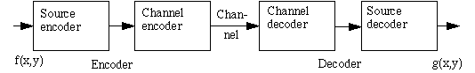
It is customary to use the names "encoder" and "decoder", which have its roots in the field of Information Theory, rather than names as "compressor" and "decompressor". If the transmission or storing channel is error-free, the channel encoder and decoder are omitted. Other wise, extra data bits can be added to be able to detect (for example parity, Cyclic Redundancy Checks) or correct (Error Correcting Code for memory) errors, often using special hardware. We shall not pay any more attention to encoders and decoders. With "lossless" compression it holds that g(x,y)=f(x,y).
A general model for a source encoder is:
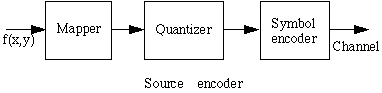 |
The "mapper" transforms the data to a format suitable for reducing the inter-pixel redundancies. This step is generally irreversible and can reduce the amount of data; used for Run Length Encoding, but not in transformations to the Fourier or Discrete Cosinus domains. |
The "quantizer" reduces the precision of the output of the mapper according to the determined reliability criteria. This especially reduced psycho-visual redundancies and is irreversible. It is therefore only used for "lossy" compression.
The "symbol encoder" makes a static or variable length of code to represent the quantizer's output. It reduces the coding redundancy and is reversible.
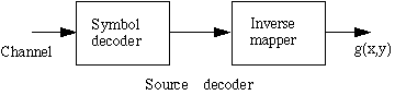 |
The general model belonging to the source decoder is shown here on the left. The inverse for the quantizer has been left out. |
Questions such as: "what is the minimum amount of data needed to represent an image" will be answered in "information theory", see chapter 8.3. The generation of information is modeled as a statistical process that can be measured in much the same manner as the intuition of information. An event E with a probability P(E) has:
I(E) = - logr P(E) r-ary units of information
P(E) = 1/2 then: I(E) = -log2 1/2 = 1 bit information
If a source generates symbols ai with a probability of P(ai), then the average information per output is:
H(z) = -
This is maximal when every symbol has an equal probability (1/N). It indicates the minimal average length (for r=2 in bits per symbol) needed to code the symbols.
For many applications this is the only acceptable manner, such as for documents, text and computer programs. This is often used for images because they are already an approximation of reality, with the spatial and intensity quantization and errors in the projection system.
Huffman coding
This is a popular method to reduce the code redundancy. Under the condition that the symbols are coded one by one, an optimal code for the set of symbols and probabilities is generated. These are:
block code: every source symbol is mapped to a static order of code symbols
instantaneous code: every code is decoded without reference to the previous symbols
and is uniquely decodable
It can be generated in the following manner. The two symbols with the lowest probability are repeatedly combined, until only two composed symbols left over. These get codes 0 and 1, the components of the composed symbol get a 0 or a 1 behind it:
Sym Prob Code Prob Code Prob Code Prob Code
a1 0.6 1 0.6 1 0.6 1 0.6 1
a2 0.2 00 0.2 00 0.2 00 0.4 0
a3 0.1 010 0.1 010 0.2 01
a4 0.06 0110 0.1 011
a5 0.04 0111
A scan from left to right of 00010101110110 results in a2a3a1a5a4.
This code results in an average 1.7 bits per symbol instead of 3 bits.
Lempel-Ziv coding
This translates variable length arrays of source symbols (with about the same probability) to a static (or predictable) code length. The method is adaptive: the table with symbol arrays is built
up in one pass over the data set during both compression and decompression. A variant on this by Welch (LZW coding) is used in the UNIX compress program.
Just as Huffman, this is a symbol encoder which can be used both directly on the input and after a mapper and quantizer.
Run Length Encoding
Many variations on this method are possible, FAX (both group 3 and 4 standards) are based on this. The run lengths themselves can be coded as independent variable length code, possibly separated for black and white if the probabilities are very different. In 2-D we can use the fact that black-white transitions in consecutive scan lines are correlated: Relative Address Coding [fig 8.17] and Contour tracing [fig. 8.18] in several varitions.
Bit plane decomposition
A gray level image of 8 bits can be transposed to 8 binary images [fig. 8.15], which each need to be coded independently by a suitable code. The most significant bits contain the longest runs and can be coded using the RLE methods. The least significant bits contain noise, here the RLE will not yield good results.
Constant area coding
The gray value image is divided into m*n large blocks which are black, white or mixed. The most probable type of block gets the code 0, the others get codes 10 and 11 and the mixed blocks are followed by a bit pattern of it. A variant is "Quadtree", where the image is divided into 4 quadrants and mixed quadrants are further divided recursively. The attained tree is then flattened.
Predictive coding
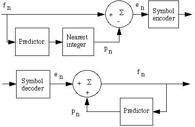 |
Starting at the previous source symbols or pixel values, the next value is predicted and only the difference with the real value is passed on. For example, the predictor can be: |
For 2-D images the rows are consecutively placed in the model above. We could also use a pixel from the previous row, for example
p(x,y)= round (a1f[x,y-1] + a2 f[x-1,y])
to make e[x,y] as small as possible; however, a good initiation will become more difficult then.
Lossy predictive coding
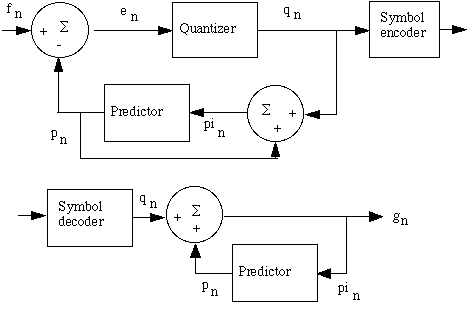 |
A quantizer, that also executes rounding, is now added between the calculation of the prediction error en and the symbol encoder. It maps en to a limited range of values qn and determines both the amount of extra compression and the deviation of the error-free compression. This happens in a closed circuit with the predictor to restrict an increase in errors. The predictor does not use en but rather qn, because it is known by both the encoder and decoder. |
Delta Modulation is a simple but well known form of it:
pn =pin with
qn =sign ( en) and can be represented by a 1-bit value: -
Disadvantages are the so-called "slope overload" because a big step in fn must be broken down into a few smaller steps ![]() , and the "granular noise" because a step of
, and the "granular noise" because a step of ![]()
![]() must be made repeatedly, see [fig 8.22].
must be made repeatedly, see [fig 8.22].
With Differential Pulse Code modulation (DPCM), pn = i=1![]() m
m ![]() i pin-i. Under the assumption that the quantization error (en-qn) is small,
the optimal values of
i pin-i. Under the assumption that the quantization error (en-qn) is small,
the optimal values of ![]() i can be found by minimizing E{en2} = E{
[fn-pn]2 } . The
i can be found by minimizing E{en2} = E{
[fn-pn]2 } . The ![]() is seem to depend on the autocorrelation
matrices of the image. These calculations are almost never done for each single image but rather for a few typical images or from models of them. See [fig 8.23 and 8.24] for the prediction error of 4
prediction functions on a given image.
is seem to depend on the autocorrelation
matrices of the image. These calculations are almost never done for each single image but rather for a few typical images or from models of them. See [fig 8.23 and 8.24] for the prediction error of 4
prediction functions on a given image.
Instead of one level, the quantizer can also be L levels step-wise: Lloyd-Max quantizers. Look at [fig 8.25], the steps can be determined by minimizing the expectation of the quantization error.
Adjusting the level ![]() (per for example 17 pixels) with a restricted amount (for example 4) scale factors
yields a substantial improvement of the error in the decoded image against a small decrease in the compression ratio (1/8 bit per pixel), see [table 8.10]. In [fig. 8.26, 8.27] the decoded images and
their deviation are given for several DPCMs.
(per for example 17 pixels) with a restricted amount (for example 4) scale factors
yields a substantial improvement of the error in the decoded image against a small decrease in the compression ratio (1/8 bit per pixel), see [table 8.10]. In [fig. 8.26, 8.27] the decoded images and
their deviation are given for several DPCMs.
Transformation coding
|
A linear, reversible transformation (such as the Fourier transformation) maps the image to as set of coefficients which are then quatized and coded. |
Often small sub-images are used (8*8 or 16*16) and small coefficients are left out or quantized in less bits. See [fig. 8.31] for DFT, Discrete Cosine Transformation and Walsh-Hadamard
Transformation with 8*8 sub-images where the smallest 50% of the coefficients are left out. The DCT is often the best of the three for natural images. See [fig 8.33], a Karhunen-Loeve Transformation
(KLT) is better but costs far more processor time. DCT also has the advantage over DFT that there are less discontinualities in the sub-images, this is less restrictive when seen by the human eye.
The coefficients can be quantized in less bits by dividing them by certain optimal values [fig. 8.37], the higher the frequency the larger the number. The DC (frequency 0) component is often treated separately by the symbol encoder because this is larger than the other coefficients.
JPEG makes use of 8*8 sub-images, DCT transformation, quantization of the coeffients by dividing with a quatization matrix [fig. 8.37b for Y], a zigzag ordering [fig. 8.36d] of it followed by a Huffman encoder, separatly for the DC component. It uses a YUV color model, the U and V component blocks of 2 by 2 pixels are combined into 1 pixel. The quantization matrixes can be scaled to yield several compression ratios. There are standard coding tables and quantization matrices, but the user can also indicate others to obtain better results for a certain image.
New developments
New developments in the field of lossy compression use fractals, see for example Fractal Image Compression and Fractal Image Encoding, or wavelets, see for example Wavelet Compression and chapter 8.5.3.
 |
 |
 |
 |
From Image Compression: GIF original Image (161x261 pixels, 8 bits/pixel), JPEG compression 15:1, JPEG compression 36:1, Fractal compression 36:1.
To store images in a file a certain format is required. Usually in the form of a header, followed by the data and possibly a trailer. The header contains information about:
Many formats are used, see Graphics/file Formats FAQ for an overview. Every application such as XITE, possibly belonging to a certain input or scanning apparatus, often uses its own format for images. Besides that they are the graphical packets with which drawings with lines, rectangles, text, etc. can be made, they usually contain "pixel map" images.
A well known "toolkit" on UNIX for the conversion between many formats is PBMPLUS. Conversion takes place to and from that own format. It can handle black∓white, gray level, colors and multi-type formats, more than 50 types!
A few well-known formats are:
Updated on February 3rd 2003 by Theo Schouten.